
-
Please try to be as accurate as possible with your search.
-
We can quote you on 1000s of specialist parts, even if they are not listed on our website.
-
We can't find any results for “”.
Pressure Transmitter Calibration Drift: Correction Methods That Actually Work
As someone who has spent a few decades commissioning and rescuing control systems in refineries, chemical plants, and power stations, I can tell you that pressure transmitter calibration drift rarely breaks things overnight. It sneaks in. A few tenths of a percent here, a little zero shift there, and suddenly you are fighting “mysterious” level alarms, off-spec batches, or compressors that never quite stay on their curves. The good news is that drift is manageable if you understand what it is, why it happens, and how to correct it with disciplined methods instead of ad‑hoc tweaks.
This article walks through practical, field-proven ways to diagnose and correct pressure transmitter calibration drift, drawing on guidance from manufacturers and metrology specialists such as Ashcroft, Fuji Electric, Honeywell, ISA, and others. The focus is not just on theory but on what works when you are standing in front of a live loop with production waiting.
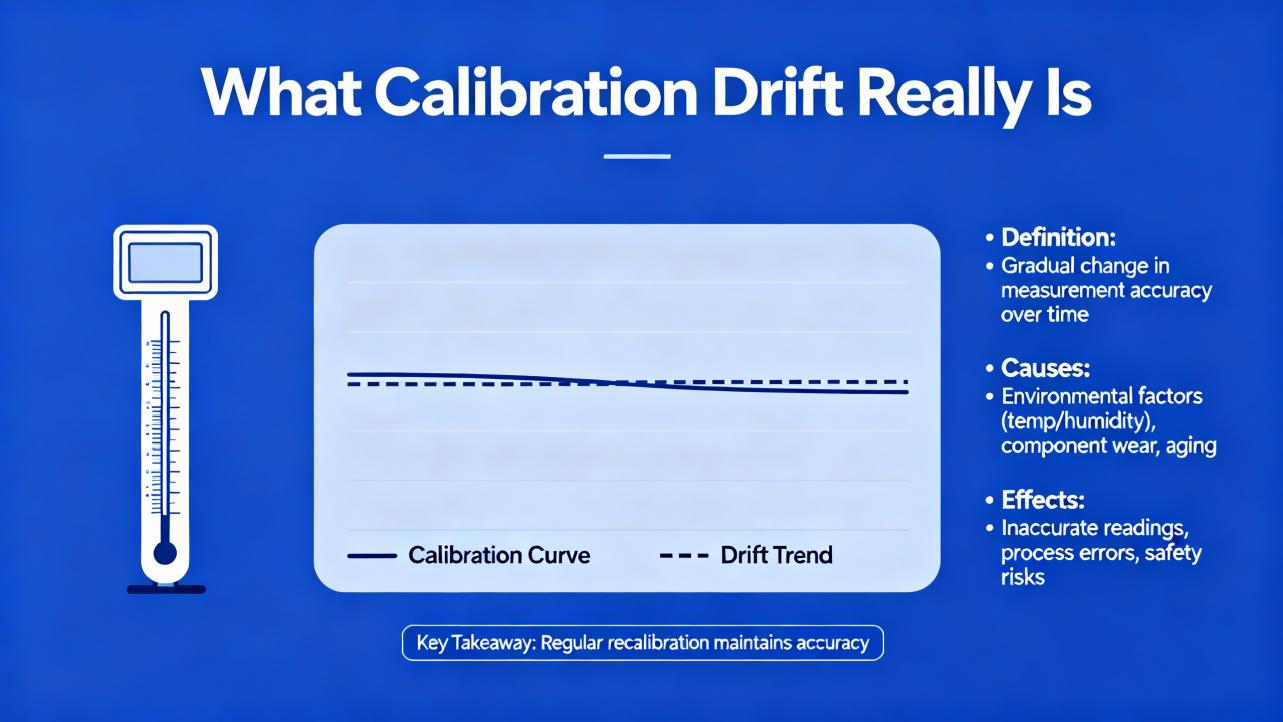
What Calibration Drift Really Is
Pressure transmitter basics
A pressure transmitter converts process pressure into an electrical signal, most commonly a 4–20 mA analog current or a digital signal on a protocol such as HART, FOUNDATION Fieldbus, or Profibus. A sensing element (strain gauge, capacitive cell, piezoresistive chip, or similar) reacts to the applied pressure, and electronics condition that raw signal into a calibrated output sent to the control system.
As one experienced engineer in an Automation and Control Engineering forum reminded a new technician, the 4–20 mA loop is only how the transmitter represents the process variable to the system. The important question is what physical range that signal is supposed to represent. It might be 0–1,000 psi for pressure, 0–50 gallons per minute for flow, or a particular temperature range. Until the physical range is clearly defined, debating milliamps does not solve the real problem.
Zero, span, and offset
Ashcroft defines two critical concepts for pressure transducers and transmitters: zero offset and span offset. Zero offset is the error at the bottom of the range when there should be no pressure (or full vacuum for some ranges). If you vent a gauge transmitter to atmosphere and it outputs 5.5 mA instead of 4.0 mA, that is zero error. Span offset is the error at the top of the range. For a 0–1,000 psi transmitter scaled to 4–20 mA, if 1,000 psi only gives you 19.5 mA, you have a span error.
Both zero and span offsets are usually expressed as a percentage of span or output. When their magnitude exceeds the device’s specified accuracy, you no longer have a reliable measurement. Correcting zero shifts the entire output line up or down; adjusting span changes its slope.
Drift versus offset and noise
Several sources, including Honeywell and multiple pressure sensor manufacturers, emphasize the distinction between drift and other error types.
Offset is a static bias. A sensor might always read 2 psi when the true pressure is zero. Drift is the gradual change in output over time when the true pressure is unchanged. For example, a 100 psi sensor with 0.5% of full-scale drift per year might shift 0.5 psi annually at constant pressure, while a high precision sensor with 0.1% of full-scale drift per year would only move 0.1 psi per year. Noise and interference, by contrast, show up as random fluctuations, not a slow, one-directional change.
EastSensor and other vendors typically specify drift as a maximum change over a given period under stable conditions. High-grade transmitters may drift less than about 0.1% of full scale over several years, while low-cost units can drift several times more. All of this drift stacks on top of any zero and span offsets you already have.
In practical terms, calibration drift is the long-term shift of the transmitter’s zero, span, or overall curve away from the original factory or last calibration, caused by aging, environmental stress, and process conditions.
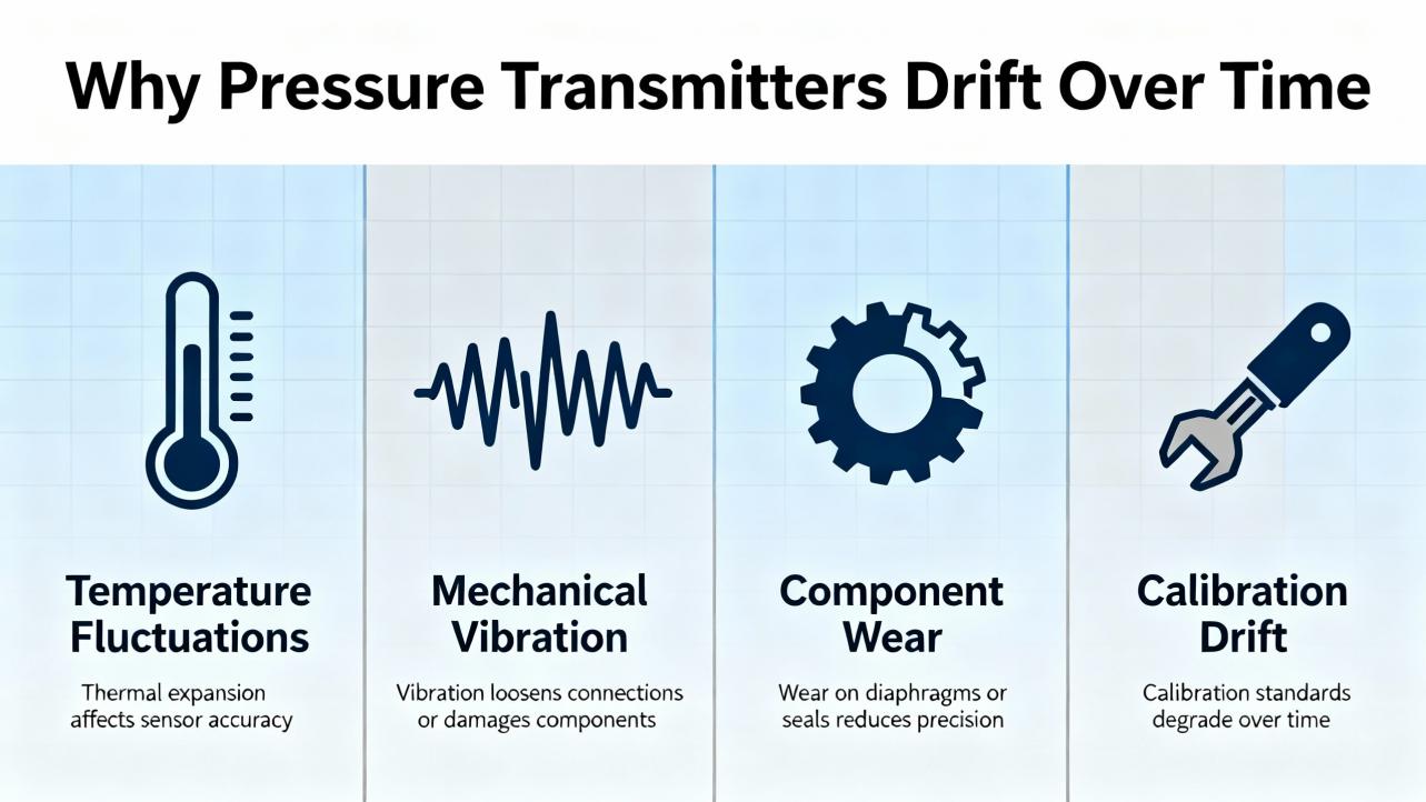
Why Pressure Transmitters Drift Over Time
Sensor and electronics aging
Pressure sensor drift is not a defect; it is a consequence of materials and time. TxSensors and other manufacturers explain that in piezoresistive devices, the diaphragm and bonding structures evolve under exposure to pressure and temperature. Adhesives cure, diaphragms flex millions of times, and internal films or strain gauges slowly change their properties. Honeywell notes similar aging in electrodes, membranes, and reference elements across sensor types.
Electronics also age. Components such as resistors and capacitors drift from their original values, and analog-to-digital converters and signal conditioners can move slightly over long periods. MeasureX and other metrology-focused sources point out that this electronics drift adds to the mechanical contributions.
High-end transmitters mitigate this with better materials, stress-relieved designs, and careful manufacturing. Fuji Electric, for example, cites long-term stability on the order of ±0.1% of upper range limit over about ten years for some of its modern transmitters. That is excellent, but not zero.
Environmental and installation factors
Honeywell highlights harsh environments as a major driver of drift. Extreme temperatures, humidity, condensation, dust, dirt, and corrosive or reactive chemicals can coat or corrode the sensing surface, change the properties of diaphragms and fill fluids, and attack housing seals. EastSensor notes that temperature variation is often the dominant factor, which is why temperature compensation is such a common design feature.
Mechanical mounting matters too. Vibration, mounting stress, and poor impulse line design introduce forces that the sensing element was not meant to see. Over time those forces deform internal parts and shift the baseline. Zero point drift can be particularly sensitive to mechanical stress, as Xidibei explains in its discussion of zero drift mechanisms.
Improper placement is another subtle contributor. A transmitter mounted close to a heat source, subjected to drafts, or located where ambient conditions swing more than necessary will experience more drift than the same model installed in a benign, temperature-controlled enclosure.
Process abuse and mechanical stress
In the field, the fastest way to ruin a good transmitter is to subject it to pressure, temperature, or media it was not designed to handle. Sources focused on troubleshooting, such as Fuji Electric and several manufacturers summarized in the research notes, list overpressure, sudden pressure spikes, and mechanical shock as frequent causes of permanent span and linearity changes.
Overpressure can permanently deform the sensing diaphragm or overload the isolating structures. Repeated high-cycle pressure swings, especially near the top of the range, accelerate fatigue. Vibration from pumps, compressors, or rotating equipment can both stress the sensor and fatigue solder joints or connections in the electronics.
Chemical exposure plays its part as well. If the wetted materials are not truly compatible with the process fluid and temperature, corrosion will first affect accuracy and eventually lead to failure. AIChE guidance on transmitter life extension emphasizes correct material selection using corrosion tables and databases to avoid this long-term degradation.
Calibration and configuration practices
Calibration practices themselves can induce or mask drift. Honeywell points out that long calibration intervals, poor procedures, or out-of-tolerance reference standards allow small errors to accumulate unchecked. ISA’s guidance on calibrating pressure transmitters warns against unnecessary sensor trims on modern transmitters, especially new ones. A “trim” in the field is usually a one-point adjustment under current conditions; overuse of trims can degrade a well-characterized factory calibration built from many points in a controlled lab.
Configuration errors often get mis-labeled as drift. Articles from Fuji Electric and Fuji’s metrology partners describe common mistakes: setting unrealistically tight maximum permissible error, using the manufacturer’s reference accuracy as the in-service tolerance, or choosing the wrong measuring range or turndown. Wrong range selection, as Fuji Electric explains in its discussion of five measurement error sources, is a major contributor to systematic error. A transmitter sized for 0–435 psi (about 30 bar) will never be a good choice for a process that later moves to a 0–4.35 psi (about 300 mbar) regime, even if you recalibrate repeatedly.
How Drift Shows Up In Real Plants
In practice, drift does not announce itself as “calibration drift.” It shows up as operations complaints, nuisance alarms, or data that no longer matches reality. Several sources, including Digicon Solutions and Honeywell, emphasize routine monitoring and comparison against trusted references to spot these symptoms early.
Typical signs include a level transmitter that slowly creeps up over weeks when the tank’s sight glass shows no real change, a discharge pressure transmitter that reads lower every month while pump curves and valve positions say otherwise, or energy balances that no longer close even though equipment performance is unchanged. In control systems with historical trending, you will often see a slow, monotonic deviation between the transmitter and a secondary reference such as a local gauge.
The table below illustrates common patterns seen in the field and the types of issues they often indicate.
| Observed symptom | Likely underlying issue | Primary correction focus |
|---|---|---|
| Reading is consistently off by roughly the same amount across the range | Zero offset or zero drift | Zero-point calibration, review ambient and mounting conditions |
| Error grows larger toward the top of the range | Span drift, possible diaphragm fatigue or electronics aging | Full span recalibration, evaluate for overpressure history |
| Different readings at same pressure when going up versus down | Hysteresis from mechanical stress or wear | Multi-point test, assess for mechanical damage, consider replacement |
| Slow, one-directional change over weeks or months | Long-term drift from aging, temperature, or environment | Trend analysis, adjust calibration interval, improve environment |
| Sudden “step” change after a process upset or event | Overpressure, impact, wiring change, or configuration change | Root-cause investigation, as-found calibration, possible replacement |
When you see these patterns, the right response is not immediately to spin the zero and span. A disciplined workflow protects you from “calibrating in” a process or configuration mistake.
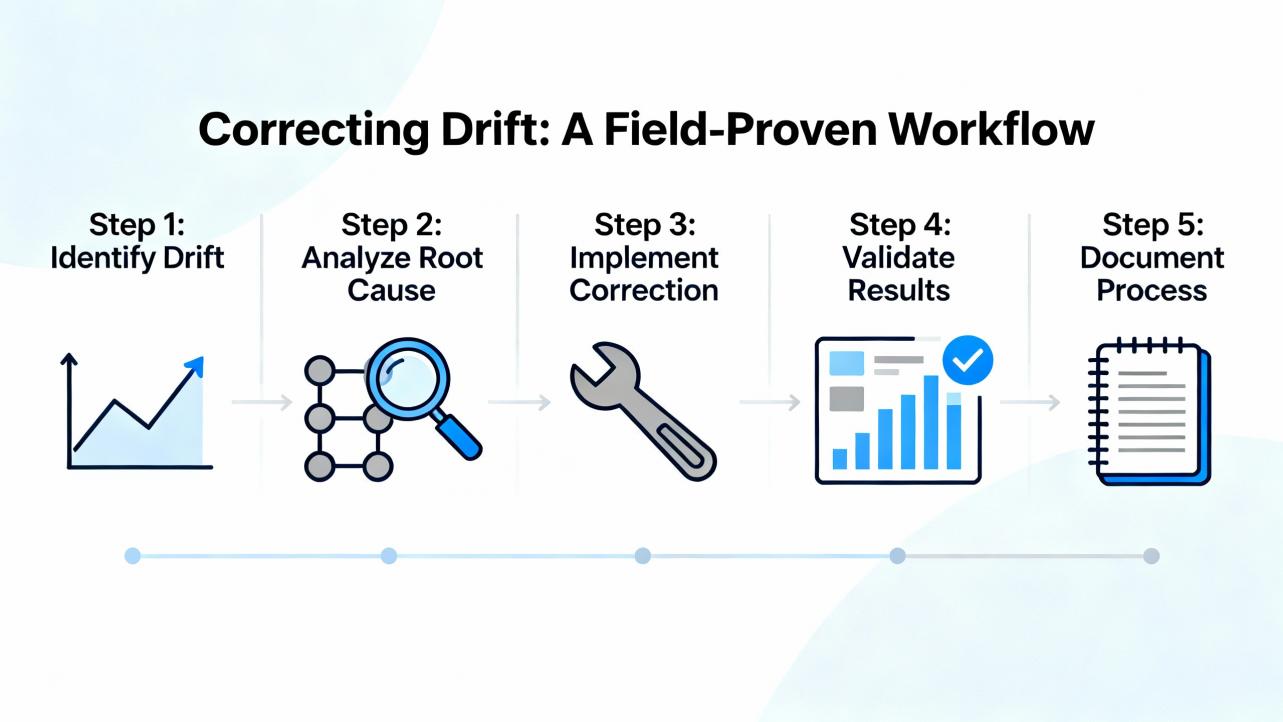
Correcting Drift: A Field-Proven Workflow
Start with the process and the loop
Before touching the transmitter adjustments, confirm what the instrument is supposed to measure and how the loop is wired. The veteran engineer on the Automation and Control Engineering forum who outlined a nine-point calibration sequence made a key point first: you must know the actual process range.
Confirm the lower and upper range values, the engineering units, and what 4 mA and 20 mA are supposed to represent in the control system. Verify power supply voltage, loop load, and polarity. Check that the right analog input or digital channel is being used and that no unintended scaling or offsets have been configured in the PLC, DCS, or data acquisition system.
Then check the process side. Use a trusted mechanical gauge or portable reference calibrator connected as close as practical to the transmitter’s pressure tap. Verify that impulse lines or capillaries are not plugged, full of gas where they should be full of liquid, or vice versa. Fuji Electric and several troubleshooting guides emphasize that many so-called calibration problems are actually impulse line issues, incorrect transmitter orientation, or changes in process conditions, not sensor drift.
Perform a proper zero and span check
Once the process and loop are verified, you can move to a controlled calibration test. CDSentec and ISA both describe a standard approach that works for most transmitters.
First, ensure the transmitter and calibration equipment have reached a stable ambient temperature. Rapid temperature changes can bias readings, especially when capillaries or fill fluids are involved. Connect a traceable pressure source and reference gauge or sensor with suitable accuracy. A good rule of thumb from ISA is that your reference should be at least three times more accurate than the device under test.
Next, perform a zero check. For a gauge pressure transmitter, vent it to atmosphere or to a known zero reference. For a differential transmitter with a nominal zero differential, equalize both sides. Allow the output to stabilize, then note the as-found reading. If necessary and allowed by your procedures, adjust the zero so that the output corresponds exactly to the lower range value.
After zero, perform a span check at a known high point in the operating range. Many plants use the upper range value; some prefer a midspan or mid-high point based on process conditions. Apply the pressure with your standard, allow stabilization, then compare the transmitter output to the expected value. Adjust span if the error exceeds the maximum permissible error defined for that instrument and service.
Crucially, do not chase tiny differences that are within your defined tolerance. ISA cautions against trying to “improve” a transmitter that is already within its allowed error band, especially with unnecessary sensor trims on modern devices.
Use multi-point characterization, not just two points
Two-point zero and span calibration is necessary but not always sufficient to see how drift has affected the entire measurement curve. Ashcroft notes that correcting zero and span changes the offset and slope, but it does not fully capture nonlinearity or hysteresis.
A practical method, echoed by both forum practitioners and formal guides, is to test multiple points across the range. One field-friendly approach is a nine-point sequence: simulate the process variable at 0, 25, 50, 75, and 100 percent of span on the way up, then back down through 75, 50, and 25 percent to 0. For each input, you record the expected and actual output. This up-and-down sequence checks both linearity and repeatability.
CDSentec describes more advanced three-point methods that fit a polynomial to typical sensor behavior, which manufacturers can use at production scale. In the plant, you rarely fit polynomials, but you can certainly examine whether mid-range points between zero and span stay within tolerance. If the ends look good but the middle does not, you are seeing nonlinearity or local deformation, not a simple zero or span drift.
Decide whether to recalibrate, re-range, or replace
Once you have multi-point data, you can make an informed decision. If the errors are reasonably linear and within your allowed maximum after a zero and span adjustment, a straightforward recalibration is appropriate. Document the as-found and as-left results for future trend analysis, as all the metrology-focused sources strongly recommend.
If the pattern shows large errors that are not corrected by zero and span, or if hysteresis is significant (different readings for increasing and decreasing pressure at the same point), you are likely dealing with mechanical wear, diaphragm damage, or internal problems. In that case, further adjustment may mask the problem rather than solve it. Articles from TxSensors, MeasureX, and troubleshooting guides agree: persistent or erratic drift, visible damage, or inability to meet specifications despite proper calibration are clear signs that replacement is the safest route.
Sometimes the transmitter itself is fine but the chosen range no longer suits the process. Fuji Electric and AIChE both present examples where the process operating range changes by an order of magnitude, making the original sensing cell and turndown a poor fit. In those cases, the correct action is to select a transmitter with a more appropriate range and rangeability rather than recalibrating the existing one endlessly.
Bench versus in-situ calibration
There is always a tradeoff between bench calibration and in-situ calibration. ISA and several industry guides note that bench calibration in a controlled environment gives you the best control over temperature, vibration, and reference quality. It is ideal when you need highly traceable results or when the process environment is particularly harsh.
On the other hand, field calibration avoids mechanical disturbances from removing and reinstalling the transmitter. Advanced transmitters, as described in the Jscepai article, support in-situ calibration with handheld communicators, high-precision digital calibrators, and even self-calibration using internal references. In hazardous or hard-to-reach areas, intrinsically safe or remote calibrators are essential.
As a systems integrator, I typically use bench calibration for critical custody transfer and safety instrumented applications, and in-situ calibration for general process transmitters where mechanical disturbance is a bigger risk than small environmental influences.
Document everything and review trends
Every reputable source, from ISA to Fuji Electric and Nagman, stresses documentation. At a minimum, record the instrument tag, location, range, as-found data, environmental conditions, reference equipment used (with certificate details), as-left data, and any adjustments made. Over time, these records let you see whether a given transmitter is stable or whether it tends to drift rapidly.
Trend analysis is not just metrology bureaucracy. Honeywell and predictive maintenance articles point out that logging and trending sensor performance allows you to move from fixed intervals to risk-based calibration. A stable indoor transmitter on a clean, steady service may justify longer intervals than a similar model outdoors in a corrosive, high-vibration application.
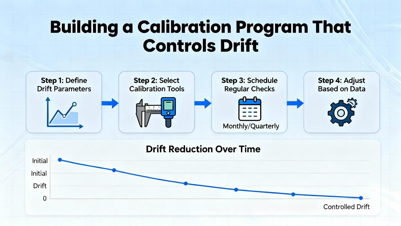
Building a Calibration Program That Controls Drift
Set realistic calibration intervals
Digicon Solutions suggests calibration every three to six months for high precision uses, every six to twelve months for general industrial service, and about annually for low-risk applications. ISA and Fuji Electric show that with modern high-stability transmitters installed indoors on stable processes, you can often extend intervals much further, in the range of several years, provided that your required in-service accuracy is not extremely tight.
Fuji Electric introduces a structured way to estimate calibration intervals using maximum permissible tolerance and long-term stability. The method looks at the required installed performance, subtracts a calculated total probable error that includes reference, temperature, and static pressure effects, and divides the result by the transmitter’s stability (expressed as drift per unit time). This gives a modeled interval before drift is likely to push the device outside its allowable tolerance. In their worked example, a high-performance transmitter with stability around ±0.1% of upper range limit over about ten years could justifiably run close to a decade without recalibration under stable conditions.
In practice, you do not start at that theoretical maximum. You begin with conservative intervals based on device class, environment, and criticality, then adjust them with real as-found data. Stable, non-critical transmitters can have intervals extended; critical or drift-prone ones may stay on shorter cycles.
Match intervals to environment and design
Fuji Electric and ISA both highlight specific factors that justify shorter intervals. Remote diaphragm seals with capillaries see more mechanical and thermal stress, so their calibration intervals are often halved compared with direct-mount transmitters. Frequent large pressure swings and overpressure events also warrant shorter intervals, because they accelerate mechanical fatigue and drift.
Location matters. Transmitters mounted outdoors in harsh climates, exposed to wide temperature swings, humidity, and contaminants, will drift faster than those in a climate-controlled instrument room. Likewise, services with dirty, viscous, or corrosive fluids place more stress on sensors and impulse lines.
Control measurement uncertainty, not just nominal accuracy
Nagman and other metrology sources remind us that calibration is about controlling measurement uncertainty, not just checking a data sheet accuracy. The total error in service includes the transmitter’s reference accuracy, its long-term stability, the influence of ambient conditions, the quality of the reference standard, and the quality of the procedure and technician performing the work.
Many manufacturers, as Ashcroft notes, use different methods such as root-sum-square or best-fit straight line when stating accuracy, which can make a device appear more precise than its real installed performance. Ashcroft’s TruAccuracy approach, for example, explicitly sums nonlinearity, hysteresis, repeatability, and zero and span offsets to represent realistic behavior.
For a calibration program that truly controls drift, you should define maximum permissible error for each instrument class based on process risk, choose reference equipment with sufficient accuracy and traceability, and ensure technicians follow consistent, documented methods.
Preventing Drift Through Better Specification and Installation
Choose the right transmitter up front
Several sources, including AIChE and Fuji Electric, make the same point: the best way to fight drift is to choose a transmitter that is appropriate for the service in the first place. That means matching wetted materials to the process fluid and temperature using corrosion tables and manufacturer selection guides, selecting an appropriate pressure range so the device operates in the middle of its span rather than at the extremes, and paying attention to rangeability so the transmitter can faithfully measure low pressures without extreme turndown.
For differential pressure-based flow and level measurements, transmitter static pressure ratings must exceed the line design pressure, and remote seals or electronic remote systems should be used when direct mounting would expose the sensor to damaging conditions. Modern multivariable transmitters that integrate static pressure, differential pressure, and temperature, as described in chemical industry articles, can also reduce the risk of mismatch between separate components.
High-quality, temperature-compensated transmitters with published long-term stability specifications cost more up front but often pay for themselves by allowing longer calibration intervals and producing fewer drift-related surprises.
Install for stability, not convenience
Installation orientation and impulse line design have a big impact on both accuracy and drift. AIChE’s guidance is very specific: for gas service, mount the transmitter above the process with impulse lines sloped back toward the line to avoid liquid accumulation; for liquid service, mount below with lines sloped so gas returns to the pipe rather than collecting at the transmitter. Avoid taps at the very bottom of pipes where solids accumulate. For steam and condensing vapors, maintain equal wet legs on both sides of a differential transmitter and protect it from live steam with drop legs and isolation valves.
From a drift perspective, good installation reduces thermal and mechanical stresses. Keeping transmitters away from hot equipment, in shade where possible, or inside temperature-moderated enclosures reduces temperature swings. Solid mounting and strain relief on impulse lines and wiring reduce mechanical stress and vibration. Shielded, grounded cables reduce electrical noise that can masquerade as drift or bias readings over time.
Protect against environment and contamination
Honeywell and MeasureX both emphasize protection from contaminants. Dust, oil, and chemicals on diaphragms or membranes change their response and may trap moisture. Regular inspection and cleaning using manufacturer-approved methods helps maintain published drift specifications. Enclosures with suitable ratings keep out moisture and corrosive atmospheres.
For sensors in harsh environments, additional protection such as filters, shields, or remote seals can isolate the sensitive elements from direct attack. In critical applications, redundant transmitters with cross-checking logic provide an early warning if one device drifts away from the others.
FAQ: Practical Questions About Calibration Drift
How often should I recalibrate pressure transmitters to manage drift?
There is no single right answer, but the ranges from reputable sources give a good starting point. Digicon Solutions suggests three to six months for high precision or safety-critical applications, six to twelve months for typical industrial service, and annual checks for low-risk duties. ISA and Fuji Electric note that modern, high-stability transmitters in stable indoor environments can often justify intervals of several years, provided the required in-service accuracy is modest and as-found results remain within tolerance. In practice, start conservatively, record as-found data, and then lengthen or shorten intervals based on the stability you actually observe.
When is recalibration no longer enough and replacement is the better option?
If a transmitter shows large or rapidly growing drift between calibration cycles, significant hysteresis between increasing and decreasing pressures, or nonlinearity that zero and span adjustments cannot correct, it is usually more economical and safer to replace rather than continue to fight it. Visible mechanical damage, diaphragm corrosion, or consistent failure to meet specifications despite correct procedures are strong indicators that the sensor is at the end of its useful life. Several manufacturers, including TxSensors and ASAP Semiconductor’s technical guides, explicitly recommend replacement once drift exceeds acceptable limits or becomes frequent.
Should I prioritize bench calibration or in-situ calibration for drift control?
Use bench calibration when you need the best possible control of environmental conditions and reference standards, such as for custody transfer, regulatory reporting, or safety instrumented functions. Calibrating in a controlled shop or laboratory minimizes ambient influences and allows more sophisticated equipment, including accredited reference standards as ISA and Fuji Electric describe. Use in-situ calibration when removing the transmitter would introduce significant mechanical disturbance or downtime, or when the process environment is representative of how the device actually operates. Modern digital calibrators, handheld communicators, and transmitters with self-calibration features make in-situ work reliable when done with good procedures.
Closing Thoughts
Calibration drift in pressure transmitters is inevitable, but it is not unmanageable. In my experience, plants that treat calibration as a disciplined, data-driven process rather than a periodic “twist the screwdriver until operations stops complaining” exercise consistently enjoy safer operation, better product quality, and less firefighting. If you define realistic tolerances, follow sound calibration methods, design for a stable environment, and let your as-found data drive interval decisions, you will keep drift under control and your pressure measurements where they belong: quietly reliable, in the background, doing their job.

References
- https://www.aiche.org/resources/publications/cep/2023/september/best-practices-extend-life-pressure-transmitters
- https://www.isa.org/intech-home/2016/september-october/departments/basics-of-calibrating-pressure-transmitters
- https://blog.ashcroft.com/what-causes-zero-and-span-offset-in-pressure-transducers
- https://atech-sensor.com/show-1883.html
- https://valveinformation.jscepai.com/fixing-pressure-transmitter-calibration-errors-expert-solutions
- https://www.kaidi86.com/a-news-pressure-transmitter-calibration-best-practices-for-accuracy.html
- https://cdsentec.com/pressure-transmitter-calibration-methods/
- https://haygor.com/blog/4-reasons-your-pressure-transmitters-fail-and-what-each-error-message-means
- https://www.zyyinstrument.com/knowledge/common-problems-and-troubleshooting-tips-for-pressure-transmitters
- https://www.asapsemi.com/blog/how-to-calibrate-and-maintain-pressure-sensors/
Keep your system in play!
Top Media Coverage
Categories


Related articles Browse All
-
 amikong NewsSchneider Electric HMIGTO5310: A Powerful Touchscreen Panel for Industrial Automation2025-08-11 16:24:25Overview of the Schneider Electric HMIGTO5310 The Schneider Electric HMIGTO5310 is a high-performance Magelis GTO touchscreen panel designed for industrial automation and infrastructure applications. With a 10.4" TFT LCD display and 640 x 480 VGA resolution, this HMI delivers crisp, clear visu...
 -
 BlogImplementing Vision Systems for Industrial Robots: Enhancing Precision and Automation2025-08-12 11:26:54Industrial robots gain powerful new abilities through vision systems. These systems give robots the sense of sight, so they can understand and react to what is around them. So, robots can perform complex tasks with greater accuracy and flexibility. Automation in manufacturing reaches a new level of ...
 -
 BlogOptimizing PM Schedules Data-Driven Approaches to Preventative Maintenance2025-08-21 18:08:33Moving away from fixed maintenance schedules is a significant operational shift. Companies now use data to guide their maintenance efforts. This change leads to greater efficiency and equipment reliability. The goal is to perform the right task at the right time, based on real information, not just ...


- Q&A
- Policies How to order Part status information Shipping Method Return Policy Warranty Policy Payment Terms
- Asset Recovery
- We Buy Your Equipment. Industry Cases Amikong News Technical Resources Why choose us
- ADDRESS
-
 32D UNITS,GUOMAO BUILDING,NO 388 HUBIN SOUTH ROAD,SIMING DISTRICT,XIAMEN
Leave Your Comment