
-
Please try to be as accurate as possible with your search.
-
We can quote you on 1000s of specialist parts, even if they are not listed on our website.
-
We can't find any results for “”.
PLC Scan Time Error Solution: Optimization Techniques
When a production line starts missing counts, overfilling hoppers, or tripping controller faults with no obvious logic error, there is a good chance you are dealing with a PLC scan time problem, not a bad rung. As a systems integrator, I have seen “mysterious” faults vanish the moment we treated scan time as a design parameter rather than an afterthought.
This article walks through how to understand PLC scan time, recognize when it is hurting you, and apply practical optimization techniques at the code, I/O, communication, and hardware levels. The goal is not just a faster number on a diagnostic screen, but a more deterministic, reliable control system that behaves predictably under real-world load.
What PLC Scan Time Really Is
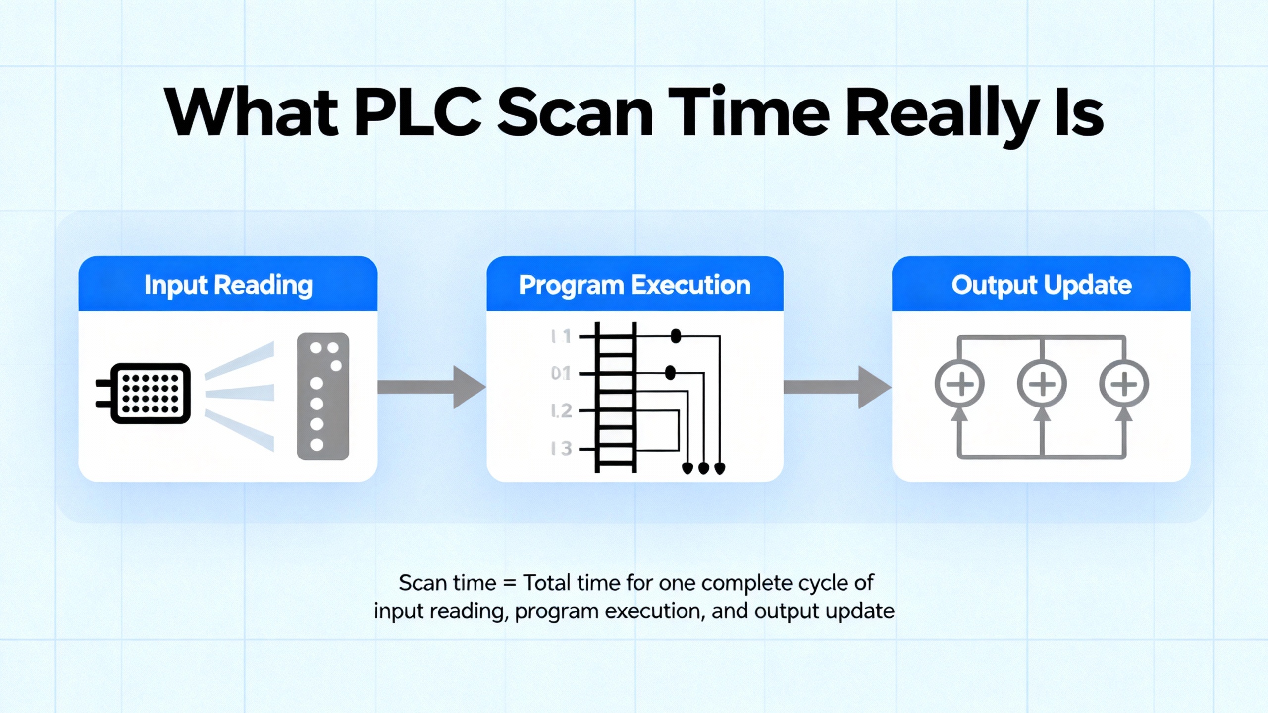
Every modern PLC executes a repeating cycle. In simple terms, it reads all inputs, executes the user program, updates all outputs, and then handles background tasks such as diagnostics and communications. The total duration of this loop is the scan time.
A technical discussion on Control.com breaks this down into three primary phases: input update, program execution, and output update. The input and output updates are mainly a function of the PLC hardware and number of I/O points. More I/O takes longer, but micro-PLCs can often complete total I/O updates in well under one millisecond. Program execution time depends on the number and type of instructions in the user logic; each instruction has a defined execution cost in microseconds that you can usually find in the manufacturer’s data.
One worked example from the same source considers an input update of about 300 microseconds, an output update of about 100 microseconds, and program instructions summing to roughly 7 microseconds. The total scan time is then about 407 microseconds. That is less than half a millisecond and extremely fast from a mechanical system’s point of view, yet still long enough to miss a very narrow input pulse if the design is careless.
Industry articles from Chief Automation and Industrial Automation Co. stress that scan time is typically measured in milliseconds and directly controls how quickly your system can react to changing inputs. Shorter scans improve responsiveness for motion control, robotics, and high-speed packaging, but chasing the absolute shortest possible scan can overload the CPU, create stability issues, and expose weaknesses in task design. At the other extreme, overly long scans cause delayed reactions, missed events, and inconsistent timing.
The right scan time is therefore not “as fast as possible” but “fast enough for the process, with margin, and consistent.”
Why Scan Time Errors Show Up in the Field
In real systems, scan time problems rarely announce themselves as “scan time too long.” Instead, they show up as watchdog faults, missed counts, or timing behavior that makes no sense until you look at the cycle time.
Industrial Automation Co. describes “Watchdog Timeout” faults on Allen‑Bradley controllers as a classic case: the program scan exceeds the configured watchdog limit, so the CPU stops for safety. Typical causes include overly complex rungs, long loops, or heavy operations that were added gradually until the controller crossed its limit.
Other errors are more subtle. A training article on PLC programming errors notes that when the scan cycle is a significant fraction of a timer’s preset, the timer can no longer track time accurately. The accumulated value is updated only once per scan, so you may never hit the exact preset or may overshoot it badly. In field terms, a “one-second” timer can become an unpredictable delay if your scan is hundreds of milliseconds and jittering.
On the sensing side, a PLC troubleshooting guide points out that input signals must be long enough relative to both the input module’s response time and the PLC scan. They recommend that the pulse be longer than the input unit’s maximum response plus roughly two PLC scans. If a sensor’s pulse is shorter than that combined interval, the PLC may never see it, no matter how perfect your ladder logic looks.
A community thread about a concrete batching plant controlled by a CLICK PLC illustrates the issue well. The system read four load cells over RS485, performed extra confirmation logic and alarm timing in ladder code, and continuously pushed weight data to a PC-based SCADA. In testing, the PLC could not close the weighing valves at the correct moment. Once the developer stripped out some confirmation logic, removed an alarm timer, reduced the SCADA update rate, and made a few mechanical adjustments, the measured scan rate improved and weighing accuracy increased dramatically. The price was losing some features the process engineer wanted, forcing a second optimization pass to regain functionality without sacrificing scan time.
Those are scan time problems in practice: logic that technically “works” but cannot run fast enough to meet process requirements.
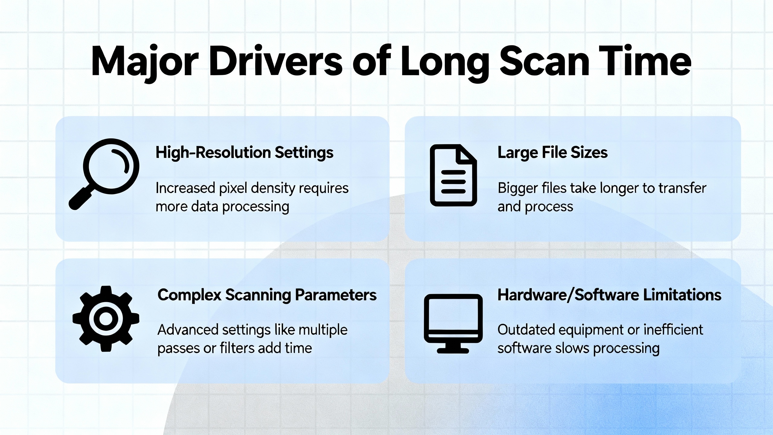
Major Drivers of Long Scan Time
Several sources converge on the same root causes for long or unstable scan times.
Program complexity is usually the first culprit. Articles from Chief Automation, Industrial Automation Co., and a LinkedIn engineering brief all highlight how large numbers of instructions, deep nesting, complex function blocks, and heavy data manipulation directly lengthen program execution. Unnecessary loops, repeated tag combinations, and overuse of float calculations are particularly expensive.
I/O design and field networks come next. Both Chief Automation and Industrial Automation Co. emphasize that more I/O modules and slower buses increase I/O latency. Traditional protocols such as Modbus over serial links add significant delay compared with faster industrial Ethernet protocols like EtherNet/IP or PROFINET. When multiple devices share a bus, as in the batching plant with four load cell amplifiers on RS485, the communication overhead becomes a significant part of each scan.
Communication traffic from HMIs, SCADA, and higher-level systems also matters. Chief Automation specifically calls out OPC UA, MQTT, and similar protocols as sources of scan-time overhead when polling rates are aggressive or tag sets are large. The CLICK PLC example shows that simply reducing the SCADA update rate can materially improve scan performance.
Data handling and memory usage are another recurring factor. Large tag arrays, extensive recipes, detailed data logging, and numerous diagnostic tags increase both memory footprint and the amount of work per scan. Chief Automation recommends routinely cleaning unused tags and maintaining organized data structures to avoid unnecessary processing.
Finally, hardware capability sets a ceiling. Chief Automation and Industrial Automation Co. both note that older or entry‑level PLCs may struggle with modern workloads, while newer multi‑core controllers handle complex, time‑critical tasks more easily. Control.com cautions, however, that marketing claims about the “fastest PLC” are meaningless unless you normalize for I/O count, program size, and clearly defined timing specs.
The table below summarizes these factors.
| Layer | How it increases scan time | Typical symptom in the field |
|---|---|---|
| Program logic | More instructions, deep nesting, heavy math and data manipulation | Watchdog trips, sluggish response, timers that feel “off” |
| I/O and networks | Many modules, slow buses like serial Modbus or RS485 | Missed short pulses, delayed reactions to sensors, jittery motion |
| HMI/SCADA comms | High polling rates, many tags, chatty protocols like OPC UA or MQTT | Scan time spikes when screens change or historians run |
| Data structures | Large arrays, recipes, logging, unused tags and variables | Gradual scan degradation as project evolves |
| Hardware | Older or low-end CPUs, limited memory, minimal comms processing capability | System performs well in tests but collapses when full load is enabled |
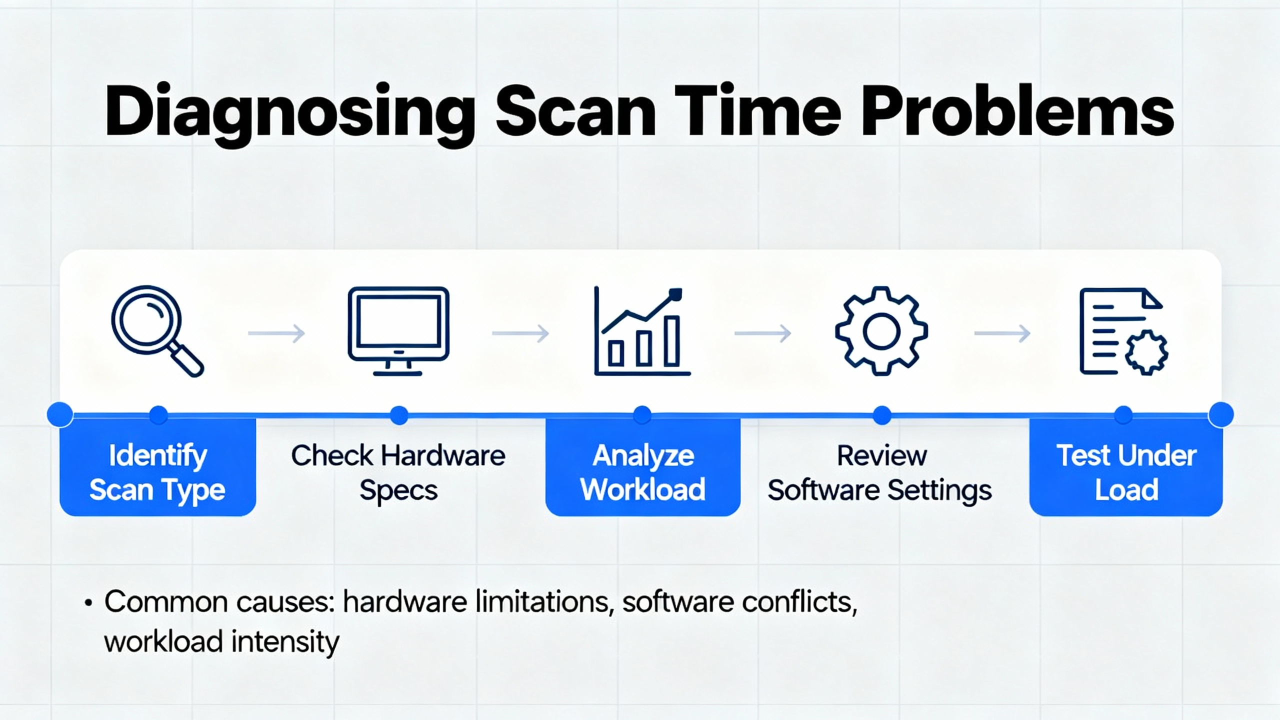
Diagnosing Scan Time Problems
Effective optimization starts with measurement. Several sources recommend using both vendor documentation and live diagnostics.
Control.com suggests a simple theoretical approach: list every instruction in your program, look up its execution time in the PLC manual, and sum them. Add the vendor’s input and output update times to get an estimate of total scan time. Because real-world events can align badly with the scan, the author recommends pessimistically doubling that calculated time when you design safety-critical sequences. For example, if an input changes just after the PLC samples inputs, it may take nearly two full scans before your output reflects it. Designing with that worst case in mind prevents surprises.
At the same time, modern PLCs expose live scan time and CPU load counters. Chief Automation and Industrial Automation Co. both recommend continuous monitoring of scan time via diagnostics, along with trending tools to catch drift or spikes. Zero Instrument’s notes reinforce the value of watching watchdog timers and setting alarms if scan time approaches configured limits or varies unexpectedly.
Testing under load is equally important. Zero Instrument recommends verifying PLC programs under worst-case conditions: all I/O active, all communications enabled, and all tasks running. Scan time must remain within your design limit under that full load, not just in a quiet commissioning environment. Chief Automation further suggests simulating program changes in a virtual environment to spot scan-time regressions before deploying them into a live plant.
Finally, pay attention to how scan time interacts with timers and counters. The PLC Technician training material points out that when the scan cycle is a substantial fraction of a timer’s preset, the timer accumulated value may never closely match the preset at any single scan, leading to apparently random actuation. Their practical recommendation is to replicate the timer rung in multiple locations so the accumulated value updates more than once per scan, effectively increasing temporal resolution without changing hardware.
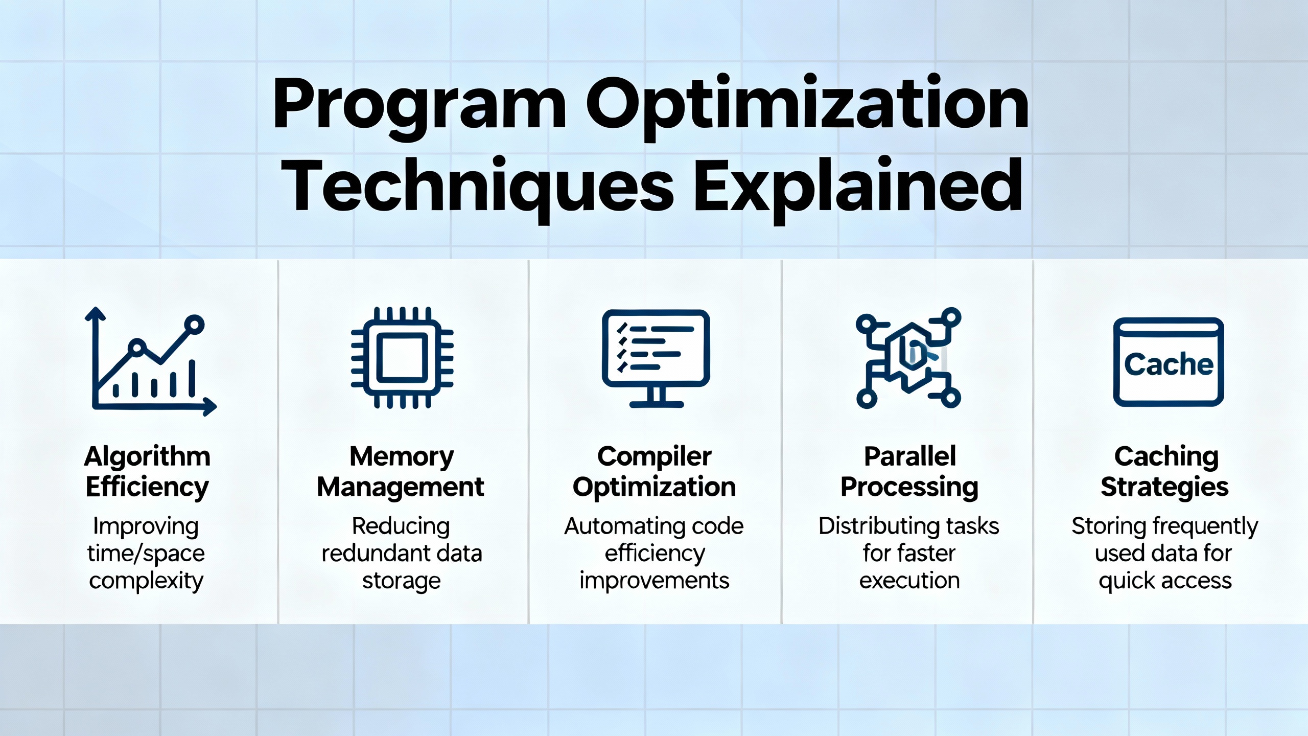
Program Optimization Techniques
Optimization should begin at the code level, where you have the most control and the least cost.
Clean Up and Simplify Logic
A PLC Technician article on scan-time reduction recommends a simple starting point: order conditions on each rung so the ones most likely to be false appear first. If an early condition is false, the processor skips evaluating the rest of the rung, reducing total work.
The same series warns against duplicating unique tag and instruction combinations across the program. If several rungs evaluate the same complex condition, refactor that condition into a single rung or subroutine and reuse it. This not only shortens scan time but also improves maintainability and reduces the risk of inconsistent behavior during changes.
The LinkedIn optimization piece adds another dimension: use efficient logic operations and data types. Simplify boolean expressions, avoid unnecessary cascaded comparisons, and choose instructions that accomplish the same goal with fewer steps. Where you must iterate, prefer clear, bounded loops or counters rather than open-ended constructs that can balloon execution time.
Chief Automation and Zero Instrument both advocate cleaning up the tag database. Remove unused variables, obsolete alarms, and dead code. Every extra instruction and tag adds to memory footprint and, often, to scan time in subtle ways.
Control Program Flow Instead of Letting It Control You
One of the biggest levers you have is controlling which parts of the program run on each scan.
The PLC Technician scan-time article demonstrates how using jump (JMP) and label (LBL) instructions can substantially reduce the number of rungs evaluated. In their example, when an Enable_Jump condition is true, execution jumps past the rungs controlling Motor 2 and Motor 3, landing on a labeled rung further down. Those skipped rungs simply do not execute in that scan. The same concept scales: you can bypass entire sections of logic that are irrelevant in a given machine mode, such as recipe loading during steady-state running.
Beyond skipping code, the same instructions can define focused “zones” that loop over a small set of rungs. The article describes creating a region bounded by JMP and LBL where the PLC repeatedly scans only the rungs needed to monitor certain inputs. Execution loops in that zone until an exit condition is satisfied, then resumes with the rest of the program. This approach keeps scan cycles tight when rapid detection of those inputs is critical.
Subroutines are another important tool. The same training material illustrates building small, reusable routines for tasks such as computing the average of two values. With JSR, SBR, and RET instructions, these routines can be called from multiple places, passing parameters in and results out. Instead of duplicating the averaging logic everywhere it is needed, you write it once and invoke it as required, shortening the effective program each scan.
A companion article on PLC programming oversights warns about a subtle trap: directly controlling physical outputs inside subroutines that execute only under certain conditions. If the subroutine turns an output on and then stops being called, that coil may remain latched even though the main program wants to change it, leading to conflicts similar to having two rungs fighting over one output. Their recommendation is to pass variables into and out of subroutines and drive physical outputs in code that always runs, so there is a single, consistent place where each output is set.
Spread Heavy Work Across Multiple Scans
Sometimes you cannot avoid heavy calculations, but you can decide when they run.
An AutomationDirect community discussion describes a PLC program that split about twenty tasks into time slices driven by a 50 millisecond timer. The idea was that only one task would run per scan, spreading heavy math across multiple cycles. In practice, many stages still executed within the same scan, creating long peaks and defeating the purpose of time-slicing.
The key insight from that thread is that stage order and jump direction determine whether work is truly distributed. If stages are forward-stacked in program order, with each stage jumping to the next, then once the first stage is active, subsequent stages may all execute within the same scan. The load collapses back into a single large block.
Reversing the order in the program while having each stage jump to the preceding one changes the behavior. When a stage turns on the next one, the CPU has already scanned past that code for this cycle. The new stage runs on the next scan, not the current one. With careful arrangement, each stage’s heavy logic runs in its own scan, and the work is naturally spread over time.
The same example shows how using pointers lets you reuse one chunk of code to handle many similar channels, such as twenty totalizers. Instead of copying the same math twenty times, you execute it once per scan with a different pointer value, dramatically shortening overall logic while still distributing computation.
The lesson is that simply dividing logic into stages is not enough. You must design stage order and control flow so that the CPU genuinely executes them across multiple scans, rather than rebuilding one big single-scan workload in a different shape.
Choose Efficient Data Types and Math
Mathematics and data representation have a measurable impact on scan time.
The LinkedIn optimization advice notes that bit-level operations tend to be more efficient than word-level operations and that integers usually execute faster and use less memory than floating‑point numbers. The PLC Technician scan-time article makes the same point concretely: floating-point (REAL) instructions consume more memory and CPU cycles than integer (INT or DINT) operations.
They offer a simple analog-scaling example. Suppose you have an analog input from 0 to 10 volts with two decimal places of accuracy, where a value such as 8.34 volts is typical. Instead of processing that as a floating-point number, you can multiply the reading by 100 at the input, converting it to an integer ranging from 0 to 1000. All subsequent math operates on integer types. Just before writing to an analog output, you scale the integer back to a REAL within the required range.
This approach keeps most of your calculations in the faster integer domain while preserving resolution. It also makes limits and ranges easier to reason about, since you are working with whole numbers.
Chief Automation further recommends reducing data volume where possible. Clean up large arrays, remove unused recipe elements, and avoid copying full structures on every scan if only a subset of fields is needed. Less data moved and manipulated per scan translates directly into shorter and more stable scan times.
Handle Timers, Counters, and Sequencers with Scan Time in Mind
Several training materials highlight that timers, counters, and sequencers can behave unpredictably when scan-time effects are ignored.
As mentioned earlier, timers whose preset is close to the scan duration can misbehave because their accumulated value is only updated once per scan. The PLC Technician recommendation to place identical timer rungs in multiple parts of the program forces the PLC to update the accumulated value more often, improving effective time resolution without changing hardware.
Counters bring another concern: overflow and underflow. The same training article notes that counter accumulated values are bounded. When they wrap around or go negative, they can fall outside expected operating ranges and trigger undesirable behavior. The author urges designers to monitor overflow and underflow bits and include explicit logic to handle wrap-around. That is not directly a scan-time issue, but in systems where the number of counts per second depends on process speed, variable scan time can interact with counter behavior in surprising ways.
Sequencers also require careful attention. The PLC Technician article on sequencer oversights explains that masking in sequencer operations affects the entire destination word, not just the “high” bits. Bits corresponding to low mask bits are forced low when the destination word is overwritten. Beginners sometimes expect unmasked bits to remain unchanged, but in reality, only bits aligned with high mask bits can take on the source word value. Preserving existing data requires deliberate use of high mask bits where you want to retain values.
The same article clarifies that the file address in a sequencer is a pointer, not the first data element. If you configure a file address such as B3:1 with a certain length, the actual data table begins at the next consecutive address, such as B3:2, and continues for the specified length. Misunderstanding this can cause off‑by‑one errors in table addressing and unexpected output patterns that complicate scan-time debugging.
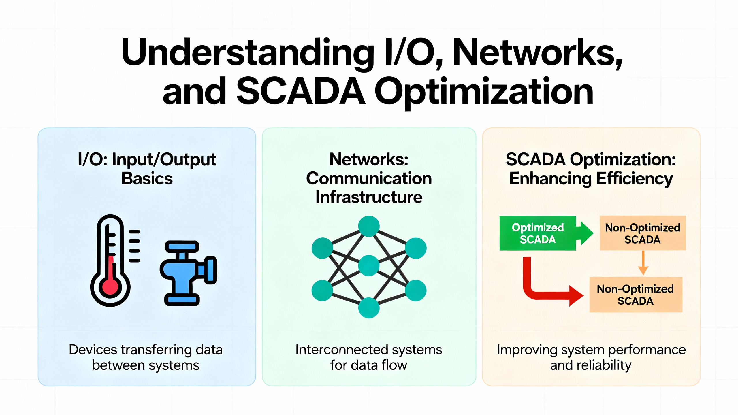
I/O, Networks, and SCADA Optimization
No matter how clean your logic is, I/O and communications can still dominate scan time.
Design I/O for Deterministic Timing
Control.com points out that input and output update times are largely fixed by the PLC hardware and number of I/O points. Micro-PLCs can read and write I/O in under a millisecond, but larger racks with many modules take longer. Manufacturers do not always publish these times prominently, yet they can usually provide them on request. For accurate scan-time estimation and process design, you should know these values.
An industrial troubleshooting article emphasizes another subtlety: input signal duration relative to scan time. For counters and step controllers to work reliably, the input signal must last longer than the input module’s maximum response time plus roughly two PLC scans. If a pulse is shorter than that combined interval, the PLC may never detect it, or detect it inconsistently.
In forum discussions about high-speed counting, practitioners sometimes attempt to solve missed pulses with interrupts or high-speed counter definitions that trigger custom functions. One such discussion shows that if the custom function itself takes too long to run, counts can still be missed, even when interrupts are used. The take‑home message is that specialized features do not remove the fundamental constraint of total processing time per event.
Tame Communication Overhead
Chief Automation and Industrial Automation Co. both highlight how communication overhead from HMIs, SCADA, and other systems influences scan time. Protocols such as OPC UA and MQTT, and industrial Ethernet links used for peer-to-peer controller communication, all compete for CPU attention and bus bandwidth.
The CLICK PLC batching plant story provides a concrete example. In addition to the load-cell math and confirmation logic, the PLC continuously transmitted weight data to a PC-based SCADA at a high rate. Four load cell amplifiers communicated with the PLC simultaneously over RS485, adding to the load. In the field, the PLC could not close the weighing valves at the correct time. After the developer removed some confirmation logic, dropped the alarm timer, and reduced the SCADA data update rate, the scan rate improved and weighing accuracy recovered.
Chief Automation advises tuning polling rates and cutting unnecessary traffic to improve responsiveness. For non-critical data such as long-term trends or infrequently used diagnostics, lower polling frequencies or batching updates can reduce scan-time impact significantly. Critical operator feedback and interlocks should remain at higher priority but still be designed with explicit knowledge of their communication cost.
The table below outlines some communication adjustments and their tradeoffs.
| Change | Effect on scan time | Tradeoff |
|---|---|---|
| Reduce SCADA/HMI polling frequency | Less CPU time spent on communication each scan | Lower temporal resolution in trends and reports |
| Consolidate data into block reads | Fewer protocol transactions per cycle | Slightly more complex mapping in SCADA or HMI |
| Move heavy analytics off the PLC | Frees CPU and scan time for control logic | Requires edge gateway or external compute resource |
| Disable nonessential diagnostic tags | Reduces data volume in each communication cycle | Less detail for ad‑hoc troubleshooting |
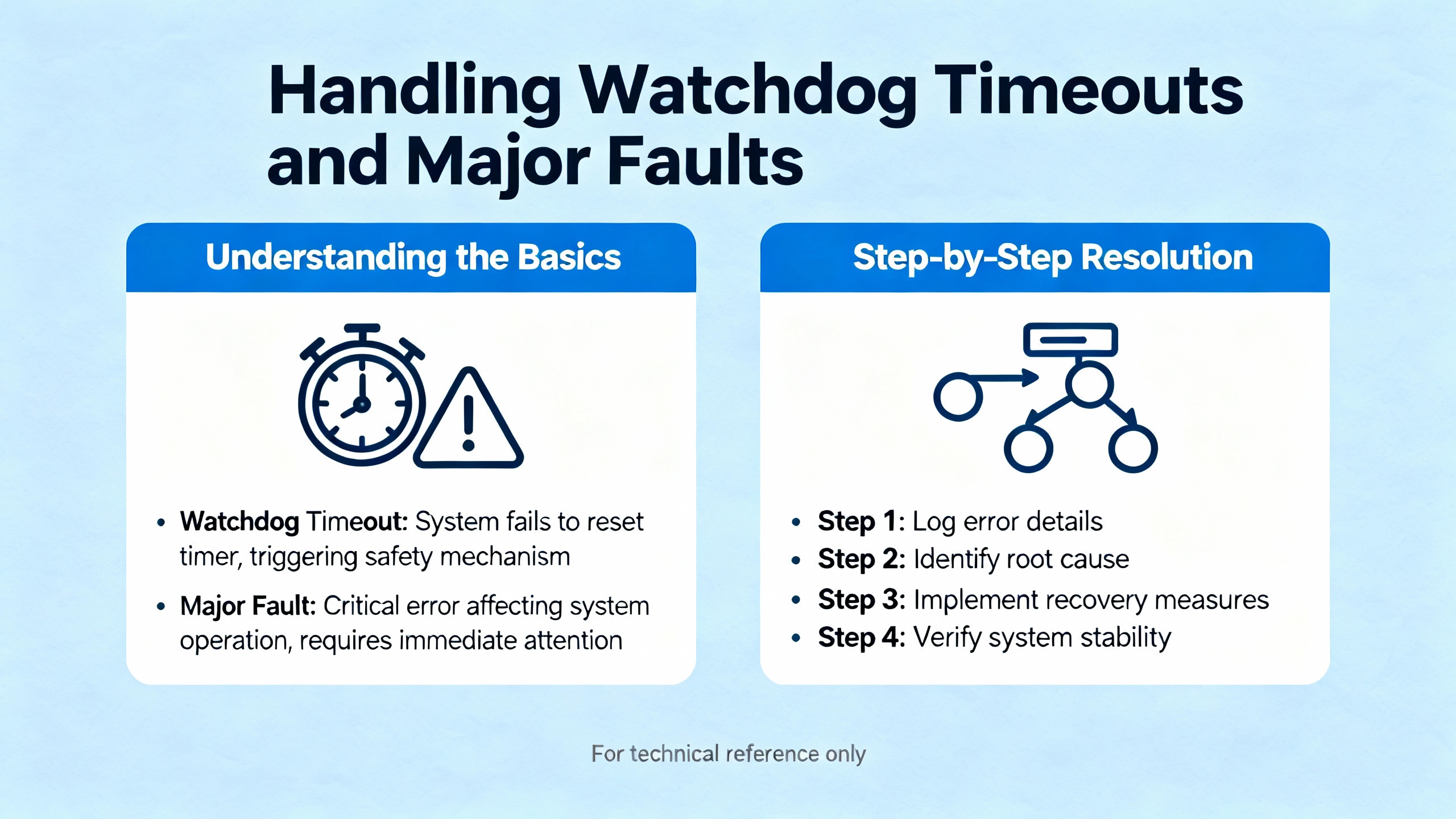
Handling Watchdog Timeouts and Major Faults
When scan time grows unchecked, the first hard symptom is often a major fault.
Industrial Automation Co. describes “Watchdog Timeout” faults on Allen‑Bradley PLCs, where the program takes longer to scan than the configured watchdog time. The controller enters a faulted state, stopping execution. Their recommended recovery path is to review the fault code in the programming software, correct the underlying logic or configuration, verify firmware compatibility, and then clear the fault and download a clean program. They also recommend simplifying and optimizing logic, eliminating infinite or long-running loops, and, if needed, upgrading to a faster CPU when scan times remain high despite optimization.
Other articles on PLC error handling echo the value of thorough diagnostics. CPU alarms, I/O alarming, and memory warnings may signal that the controller is overloaded or dealing with noise-related issues that indirectly affect scan performance. Systematic troubleshooting from inputs through program execution to outputs, using input LEDs, multimeters, and the vendor’s monitoring tools, helps distinguish scan-time issues from wiring or device faults.
The key is to treat a watchdog trip as a symptom of design overload, not just a nuisance to be cleared. Once you have the controller running again, record the maximum scan time, identify which features were recently added, and work methodically through code and communication optimizations before returning the system to full production.
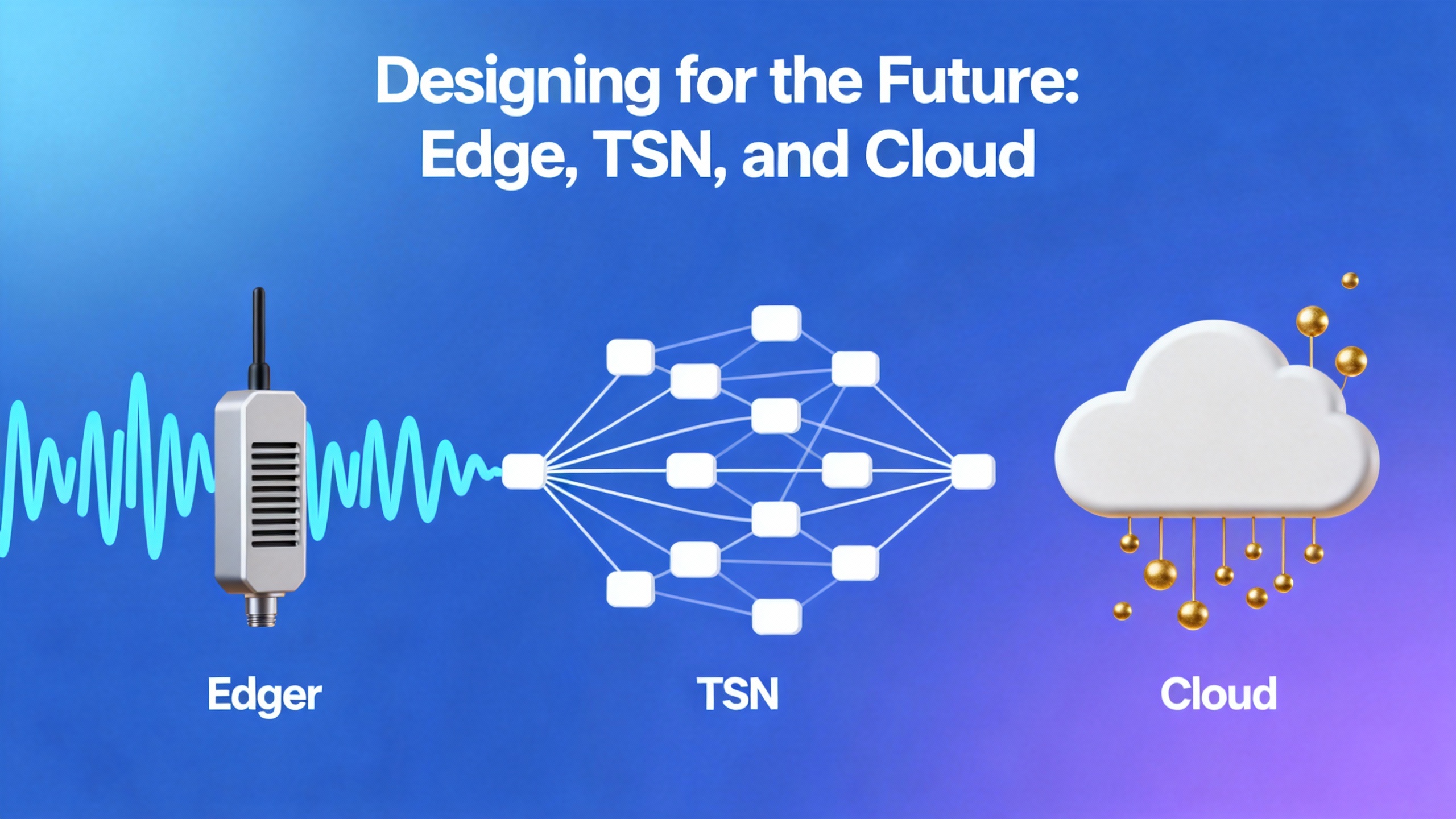
Designing for the Future: Edge, TSN, and Cloud
Scan-time management is becoming more challenging as plants embrace digitalization.
Chief Automation and Industrial Automation Co. both point to emerging trends such as edge computing, lightweight AI or machine learning on PLCs, and increased cloud connectivity. These features add computational and communication load on controllers that were originally designed primarily for deterministic control.
Time-Sensitive Networking (TSN) is one response to this challenge. By making Ethernet-based protocols more deterministic, TSN helps ensure that control traffic gets predictable timing even when the network carries non-control data as well. This does not reduce the CPU time required to execute logic, but it does tighten the overall timing budget from sensor to actuator.
At the same time, cloud connectivity introduces longer-latency, less predictable communication paths. Both Chief Automation and Industrial Automation Co. stress the need to keep these cloud interactions from affecting core scan time. Offload heavy analytics and history to edge devices where possible, and ensure your PLC treats cloud communication as a background activity with clear time limits.
Zero Instrument notes that deterministic, well-characterized scan cycles support compliance with industrial safety and reliability standards, which often require documented maximum response times to faults and process upsets. In that context, scan time optimization is not just about performance; it is part of your safety case.
A Practical Workflow for Fixing a Scan Time Error
When you encounter a scan time error or suspicious timing behavior on a project, start by capturing the facts. Record the PLC’s reported average and maximum scan times under normal and worst-case operating conditions, along with any watchdog or CPU fault codes. Check the hardware manual for instruction execution times and input/output update times, and perform a quick back-of-the-envelope estimate of expected scan time, doubling that value for a conservative design bound as suggested by Control.com.
Next, identify obvious heavy hitters in your logic and communications. Look for deeply nested rungs, large data handling sections, frequent floating-point operations, and extensive SCADA polling. Apply code-level optimizations first: reorder conditions on rungs, remove duplicated logic, consolidate calculations into subroutines, and convert suitable math to integer-based scaling. Use JMP and LBL to skip entire blocks of code that do not apply in the current machine mode, and use subroutines for repeated functions.
Then address I/O and communication. Verify that high-speed inputs have pulses longer than the combined input response and scan criteria recommended in PLC troubleshooting guides. Slow non-critical SCADA polling, consolidate data reads, and temporarily disable nonessential diagnostics while you measure the impact on scan time. In systems like the CLICK batching plant, you may find that a modest reduction in update rate recovers enough performance to reintroduce important confirmation logic reliably.
Finally, reassess whether the hardware is appropriate. If after optimization, scan time still approaches your design limit under full load, consider moving heavy non-control tasks to an edge gateway or upgrading to a more capable PLC. As Industrial Automation Co. notes, that decision should be driven by clear performance measurements, not just processor clock speed on a marketing sheet.
FAQ
How fast should my PLC scan be?
There is no single “correct” scan time. The Control.com example shows a scan of about 407 microseconds, which is extremely fast, while other systems operate comfortably with scans in the several millisecond range. What matters is that the total time from input change to output action comfortably meets process requirements under worst-case conditions, including the possibility that an input changes just after being sampled. For safety-related functions, the Control.com guidance to design with roughly double the calculated scan time as margin is a sensible starting point.
Will a faster CPU automatically solve scan time problems?
Not necessarily. Industrial Automation Co. cautions that overall scan time is influenced heavily by program complexity, I/O configuration, communication overhead, and memory usage, not just processor speed. Upgrading to a newer, multi-core PLC can certainly help with complex, time-critical tasks, but only if the program has been written and structured to take advantage of that capability. It is more effective to streamline code, reduce unnecessary data handling, and optimize communications first, then justify hardware upgrades based on measured gaps.
Can I ignore scan time in slow, non-motion applications?
Even in apparently slow processes, scan time still matters. The PLC Technician training material shows that timers can misbehave when scan time is a significant fraction of their preset, and PLC troubleshooting guides point out that counters and step controllers need inputs that last longer than input response plus two scans. Ignoring scan time can therefore produce erratic timing, miscounts, and intermittent faults even in simple processes. Treat scan time as a design parameter for every project, adjusting the level of rigor to the risk and complexity of the application.
Closing Thoughts
Scan time errors are not exotic; they are the predictable result of pushing a control system beyond what its cycle time and architecture were designed to handle. The good news is that most problems can be solved with disciplined program design, thoughtful I/O and communication choices, and measured use of modern hardware capabilities. When you treat scan time as a first-class requirement from specification through commissioning, you end up with systems that not only run faster, but run the way operations expects them to, day in and day out.

References
- https://trace.tennessee.edu/cgi/viewcontent.cgi?article=14907&context=utk_gradthes
- https://reclaim.cdh.ucla.edu/_pdfs/virtual-library/l3ZYcj/Plc_Scan.pdf
- https://www.plctalk.net/forums/threads/how-to-reduce-scan-time-of-plc.18925/
- https://www.plcacademy.com/scan-time-of-the-plc-program/
- https://www.plctechnician.com/news-blog/5-tips-how-reduce-scan-time-using-ladder-logic-part-2
- https://triplc.com/smf/index.php?topic=1112.0
- https://zeroinstrument.com/understanding-plc-scan-cycles-in-industrial-automation/
- https://community.automationdirect.com/s/question/0D53u00004d97v1CAA
- https://chiefautomation.com/blogs/news/d?srsltid=AfmBOop169KV2KnDtbVsNuJSHy6zOgfUqDsAwxe233irPnfjpw-tored
- https://www.rowse-automation.co.uk/blog/post/how-to-optimise-plc-scan-time
Keep your system in play!
Top Media Coverage
Categories


Related articles Browse All
-
 amikong NewsSchneider Electric HMIGTO5310: A Powerful Touchscreen Panel for Industrial Automation2025-08-11 16:24:25Overview of the Schneider Electric HMIGTO5310 The Schneider Electric HMIGTO5310 is a high-performance Magelis GTO touchscreen panel designed for industrial automation and infrastructure applications. With a 10.4" TFT LCD display and 640 x 480 VGA resolution, this HMI delivers crisp, clear visu...
 -
 BlogImplementing Vision Systems for Industrial Robots: Enhancing Precision and Automation2025-08-12 11:26:54Industrial robots gain powerful new abilities through vision systems. These systems give robots the sense of sight, so they can understand and react to what is around them. So, robots can perform complex tasks with greater accuracy and flexibility. Automation in manufacturing reaches a new level of ...
 -
 BlogOptimizing PM Schedules Data-Driven Approaches to Preventative Maintenance2025-08-21 18:08:33Moving away from fixed maintenance schedules is a significant operational shift. Companies now use data to guide their maintenance efforts. This change leads to greater efficiency and equipment reliability. The goal is to perform the right task at the right time, based on real information, not just ...


- Q&A
- Policies How to order Part status information Shipping Method Return Policy Warranty Policy Payment Terms
- Asset Recovery
- We Buy Your Equipment. Industry Cases Amikong News Technical Resources Why choose us
- ADDRESS
-
 32D UNITS,GUOMAO BUILDING,NO 388 HUBIN SOUTH ROAD,SIMING DISTRICT,XIAMEN
Leave Your Comment