
-
Please try to be as accurate as possible with your search.
-
We can quote you on 1000s of specialist parts, even if they are not listed on our website.
-
We can't find any results for “”.
Designing Encoder Feedback with a 100 kHz Pulse Counter Module
In real plants, encoder feedback is either rock solid or it is the silent killer of throughput and quality. Over the years commissioning motion systems, conveyors, and meters, I have learned that the difference often comes down to one component that rarely gets the spotlight: the high‑speed pulse counter module. A 100 kHz pulse counter designed for encoder signals sits right at the edge of what your mechanics can do and what your controller can actually see.
This article walks through how a 100 kHz pulse counter module works in encoder feedback applications, how to size and apply it, where it shines, and where it will bite you if you treat it like an ordinary PLC input. The discussion leans on vendor material from Maple Systems, Dewesoft, Viox, Wayjun, Solidotech, and others, combined with the hard lessons you only get on live machines.
Why High‑Speed Pulse Counters Matter
Digital encoders and pulse sensors convert motion or process events into square‑wave pulses. Dewesoft describes these as discrete on/off signals that often need to be captured in tight sync with the process. Rotary encoders on motors, linear encoders on cut‑to‑length systems, proximity sensors counting parts, and flow meters with K‑factors in pulses per gallon all fall into this family.
The reason you need a high‑speed counter is simple. A normal PLC input updates at the pace of the PLC scan. As Maple Systems points out, that scan‑rate input often “will not have the scan cycle that will allow [you] to count these signals.” You might be scanning every 10 or 20 ms; meanwhile, your encoder may be toggling hundreds or thousands of times per second. You can easily miss most of the edges.
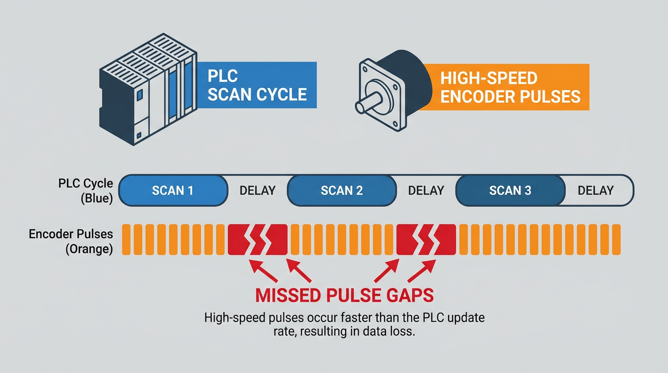
A high‑speed pulse counter (also called a high‑speed counter or HSC) sidesteps this by counting edges in dedicated hardware. Maple Systems describes high‑speed inputs that typically handle up to about 100 kHz. Dewesoft gives an example where a modest 360 pulses per revolution encoder at 600 RPM produces about 3,600 Hz; that is trivial for a proper counter, but already risky if you try to sample it purely in ladder logic.
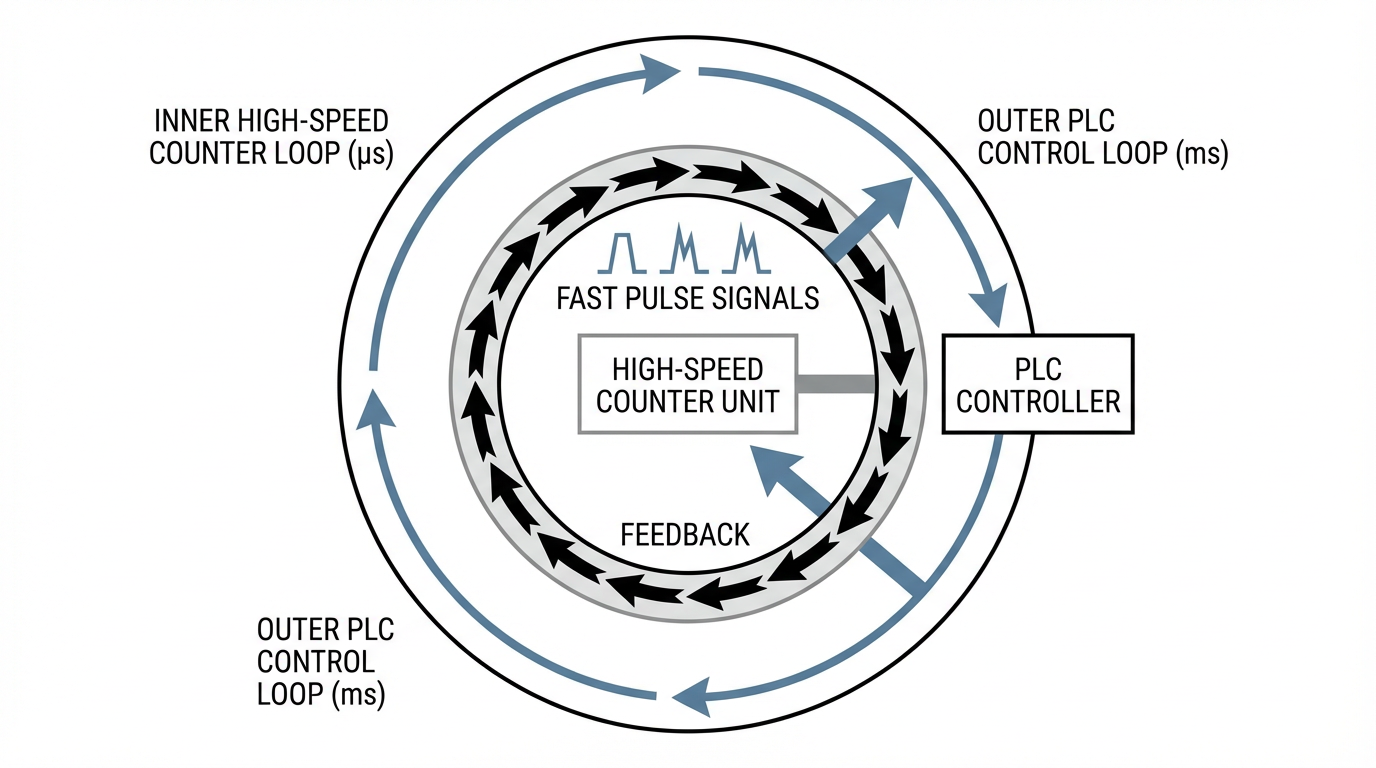
In practice, that means the module sits in the “inner loop,” watching the encoder transitions in microseconds, while the PLC or controller runs a slower “outer loop.” A Control.com discussion of Schneider high‑speed counter modules describes this explicitly: the HSC runs an inner loop at the pulse rate (in their example, 3 kHz with a module rated to 60 kHz), while the PLC runs an outer control loop at 100 ms. The rule of thumb there is that the inner loop should be at least twice as fast as the outer loop; in most real systems it is orders of magnitude faster, which is the whole point.
For encoder feedback applications, that inner loop is what protects you from lost counts, jittery position, and mysterious scrap.
What a 100 kHz Pulse Counter Module Actually Does
From a control engineer’s perspective, a 100 kHz pulse counter module does three jobs.
First, it receives fast digital signals from encoders or pulse sensors. In the industrial world this is usually at 24 V levels. Solidotech’s pulse counter module, for example, is designed explicitly for 24 V inputs and supports both NPN (sinking) and PNP (sourcing) outputs. That is exactly what you want when tying into common incremental encoders or proximity sensors.
Second, it counts edges and possibly interprets direction. Viox’s guide to pulse counters explains that a counter generally detects rising and/or falling edges on one or more channels and maintains a signed count. Speedgoat’s pulse counter description is a typical example: a signed 31‑bit register that can increment or decrement based on the chosen count mode, with options to use rising edges, falling edges, or both.
Third, it applies signal conditioning and exposes the result to the control system. Viox emphasizes features like debounce and glitch filters to reject mechanical bounce and noise. Wayjun’s WJ150‑485 encoder interface adds configurable input filtering for mechanical contacts, plus automatic non‑volatile saving of the count so position survives a power fail. From the controller’s perspective, you no longer deal with raw pulses; you read clean counts, rates, or scaled engineering units via PLC tags, Modbus registers, or a similar interface.
In a 100 kHz class module, all of that has to keep up with pulses as close together as about 10 microseconds. That is not exotic compared with modules rated at 1 MHz (Solidotech again) or counter inputs in DAQ systems that Dewesoft notes can handle pulse bandwidths around 10 MHz, but it is fast enough that you cannot fake it in the PLC scan.
Signals, Voltage Levels, and Wiring
You only get correct counts if you get the wiring and signal levels right, and this is where I still see a lot of downtime caused by simple mistakes.
Most industrial encoder and pulse sensors are 24 V devices with either NPN or PNP outputs. The Solidotech module explicitly supports both at 24 V, which is typical for motion‑control counter modules. Wayjun’s WJ150‑485 caters to incremental encoders and discrete sensors with NPN, PNP, push‑pull, and TTL outputs, again on a wide 8–32 VDC supply.
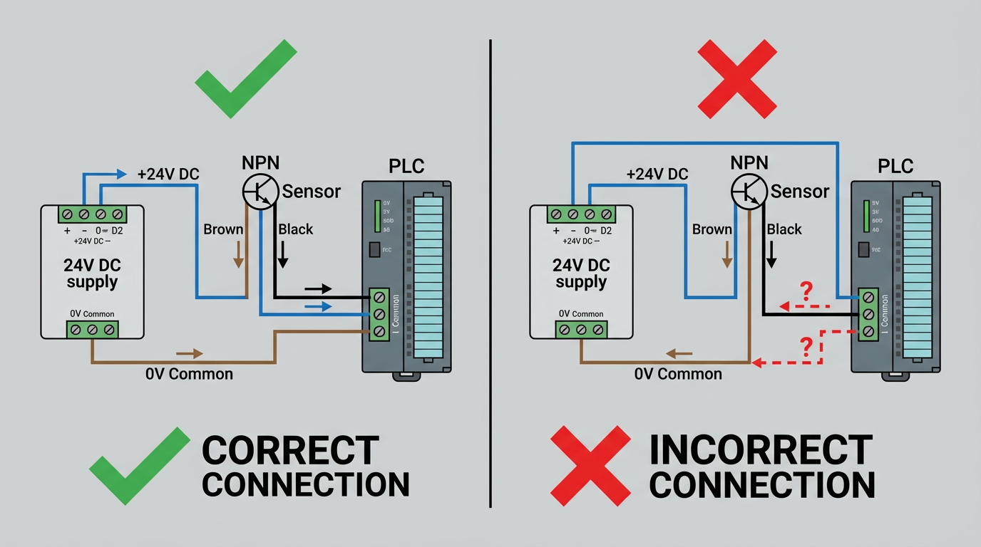
The details matter. In an AutomationDirect forum thread on a CLICK PLC pulse counter, the flow meter had an NPN transistor output. The correct wiring required tying the PLC common terminal to the positive 24 V supply. Mis‑wiring the common left the input circuit dead, and of course nothing counted until that was corrected. That is a classic trap: an NPN sensor in a sourcing input configuration will never register.
On top of proper polarity and commons, you need to think about noise. Viox, Speedgoat, and Wayjun all stress debounce and filtering. Mechanical contacts such as reed switches and some low‑cost flow meters generate very narrow spurious pulses. Viox describes using glitch filters that ignore pulses shorter than a configured time. Wayjun recommends specific filter settings for applications like rain gauges and mechanical water meters so that switch bounce does not turn one physical event into several counts. Speedgoat calls out configurable debounce as critical in electrically noisy or impedance‑mismatched wiring.
In encoder feedback applications, especially where the encoder runs at significant speed, you generally want to combine proper shielding and grounding in the cable with a realistic minimum pulse‑width filter in the module. That way, you keep your 100 kHz capability but ignore the microsecond‑level glitches that are not real motion.
Counting Modes and Quadrature Encoders
Encoders rarely just spit out a single pulse train. Incremental rotary encoders usually have at least two channels, A and B, in quadrature, and often a Z index. Dewesoft explains that these A and B channels are square waves shifted by 90 degrees, which lets you infer direction and increase resolution.
High‑speed counters expose several counting modes to take advantage of that. Maple Systems describes them in simple terms:
A single‑phase or “1x” mode counts only rising edges of one channel. A “2x” mode counts both rising and falling edges of that channel, effectively doubling the resolution. Quadrature “4x” mode uses both A and B channels, counting all transitions on both. That gives up to four counts per encoder cycle, and by checking which channel leads, the counter can tell whether the encoder is moving forward or backward.

Contec’s motion control notes describe the same thing from the motion board side: pulse outputs are either two separate lines for clockwise and counterclockwise or one pulse plus a direction bit. Fuyumotion’s motion‑control article reinforces these conventions and recommends using the two‑pulse mode for less experienced users because it is easier to understand and troubleshoot.
The 100 kHz limit of your module applies to each channel’s pulse frequency. So, if your encoder runs near that edge and you turn on 4x quadrature decoding, your effective edge rate on the counter can approach that limit quickly. That is why the module’s frequency rating and the encoder’s pulses per revolution must be considered together.
Sizing a 100 kHz Counter for an Encoder
You do not pick “100 kHz” out of a catalog and hope for the best. You size the module against your encoder’s pulse rate, including any multiplier from counting mode, and then consider resolution and sampling strategy.
The raw pulse rate is set by the encoder pulses per revolution and the shaft speed. Dewesoft gives a simple example where a 360‑pulse encoder at 600 RPM produces about 3,600 pulses per second. As they note, any counter with a bandwidth of several kilohertz handles that comfortably. Maple Systems notes that high‑speed inputs typically support up to about 100 kHz, so even with 4x quadrature, that 360‑pulse encoder is far from the limit.
At the other end, Solidotech’s module is rated to 1 MHz, so it can cope with much higher resolution encoders or higher shaft speeds. Wayjun’s WJ150‑485 sits in the middle with a 50 kHz specification, making it suitable for moderate speeds and counts, especially when you remember that it may be used in 1x mode for some applications.
On top of the raw pulse rate, you must think about the outer loop that consumes that data. On Control.com, the Schneider M340 case study has an HSC rated to 60 kHz easily handling a 3 kHz signal while the PLC reads its results every 100 ms. That is the ideal arrangement: the counter’s inner loop is fast enough to be effectively continuous, and the PLC outer loop simply polls the derived values.
In flow and process applications, the sampling window length is just as important as the frequency capability. In the AutomationDirect CLICK PLC example, a flow meter with a K‑factor of about 4,994 pulses per gallon at a maximum flow of 5 gallons per minute produced around 416 Hz. At a 100 ms sample period, you only see about 41 or 42 pulses per window. The author in that thread correctly points out that this may give poor resolution at low flows and suggests a one second window. The takeaway is that a 100 kHz module can easily track the pulses, but your choice of sampling interval and scaling in the PLC will drive the actual resolution and responsiveness seen by the process.

Translating Counts into Engineering Units
No operator cares about “pulses.” They care about inches, feet, gallons, or parts. The translation comes from a scaling factor, and this is where pulse counters start to feel like instruments rather than raw logic blocks.
Viox’s full guide to pulse counters emphasizes that you configure a scaling factor such as pulses per gallon or pulses per kilowatt‑hour and then have the counter expose scaled engineering units. Econtroldevices’ article on impulse counters describes using counts to measure length and operations, for example cutting materials to length or tracking machine cycles for maintenance.
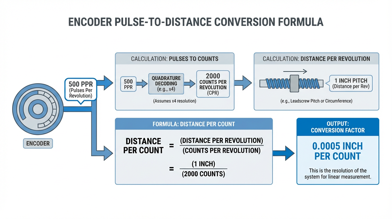
In encoder feedback, you normally know the pulses per revolution, and you know how far one revolution moves your load. Fuyumotion walks through this with a general “pulse constant” concept: pulses per revolution divided by distance per revolution gives pulses per unit distance. Using imperial units, if your screw advances 1.0 in per revolution and your encoder is 500 pulses per revolution in quadrature at 4x, you have 2,000 counts per in. That means each count is about half a thousandth of an inch.
If you store the count in a 31‑bit signed register, as Speedgoat describes, you have plenty of range before overflow.
The same thinking applies to flow meters. In the AutomationDirect example, the K‑factor of about 4,994 pulses per gallon tells you how many pulses you expect for each gallon that passes. Read the total pulse count from your 100 kHz module, divide by 4,994, and you have total gallons. Read counts over a known time window and you have gallons per minute.
What matters is that the pulse counter module gives you reliable, loss‑free pulse counts, and your PLC or controller does the arithmetic in whichever engineering units your operators understand.
Architecture: Let the Counter Module Do the Fast Work
One of the consistent recommendations from practitioners is to let the pulse counter module handle all pulse‑related calculations and let the main CPU read processed values. The Control.com discussion states this directly: rely on the high‑speed counter module to do the pulse work rather than trying to re‑implement high‑speed counting in CPU logic.
Maple Systems makes the same point from a PLC programming perspective. Their high‑speed counter feature captures the state of the inputs independently of the normal scan. You then configure it using their MapleLogic software as a special program: selecting linear or ring counters, one‑phase or two‑phase inputs, and enabling compare outputs to generate events when counts reach thresholds. The PLC logic then reads the HSC’s state and acts on it, instead of racing the scan cycle against the encoder.
Dedicated modules such as the Wayjun WJ150‑485 take this even further by moving the counter into a stand‑alone RS‑485 device. The module decodes AB quadrature, maintains a count up to roughly 20 billion, saves it in non‑volatile memory on power fail, and exposes it as Modbus data. The PLC does not see pulses at all; it sees signed counts and can even command resets or mode changes over the network.
DAQ‑oriented hardware follows a similar pattern. Dewesoft’s counter inputs run from a high‑frequency timebase and produce position, frequency, and derived quantities like RPM internally. Speedgoat’s configurable pulse counters, integrated into Simulink, implement edge selection, up/down modes, and debounce in the I/O module; the real‑time application just reads a register.
From a systems integrator standpoint, this architecture has clear advantages. The fast, fragile work is handled in a small, well‑tested block with a clearly specified frequency rating like 100 kHz or 1 MHz. The slower but more complex PLC code focuses on control algorithms, safety, and HMI, reading clean data from the module at a comfortable scan rate.
Pros and Cons of 100 kHz Pulse Counter Modules
A 100 kHz pulse counter module hits a sweet spot in many encoder feedback applications, but it is not universally ideal.
On the plus side, Maple Systems’ note that high‑speed inputs typically handle about 100 kHz tells you this is a capability level that has become standard in industrial PLC and I/O platforms. For many encoders on moderate‑speed axes, and for most flow meters and cut‑to‑length wheels, the pulse rate is comfortably below 100 kHz even when you use quadrature 4x decoding. The module remains relatively simple to configure, and the hardware cost is usually lower than the specialized 1 MHz or multi‑MHz counters you see in high‑speed test systems like those described by Dewesoft.
A 100 kHz module also tends to integrate well with mainstream 24 V encoder hardware. The Solidotech module’s 24 V input level and NPN/PNP compatibility are typical; you rarely need level shifting or additional isolation for standard factory encoders. The logic in these modules is proven for industrial environments and is supported by features like filtering, compare outputs, and non‑volatile storage, as Viox and Wayjun both emphasize.
On the negative side, 100 kHz sets an upper bound that you can hit surprisingly quickly if you stack high encoder resolution, high speed, and 4x counting. High‑resolution encoders used in precision motion systems can easily produce pulse rates that push beyond this range on fast moves. When that happens, you risk missed counts and subtle errors that only show up as angle or position drift.
Another limitation is that pulse counter modules by definition handle pulse trains. Dewesoft makes an important distinction between incremental encoders, which output pulses, and absolute encoders, which output multi‑bit digital codes over serial or fieldbus interfaces. Absolute encoders are not compatible with pulse‑based counter channels. If your application must know absolute position immediately at power‑up, not just relative motion since homing, a simple 100 kHz pulse counter will not be enough; you will either need an absolute encoder interface or a hybrid scheme.
Finally, there is the integration overhead. Stand‑alone modules like the Wayjun WJ150‑485 bring tremendous flexibility with Modbus RTU, dual modes, and deep filtering options, but they also add configuration steps, serial network design, and device management compared with a PLC’s built‑in HSC.
Common Pitfalls in Real‑World Deployments
In the field, the same failure modes surface repeatedly when teams add encoder feedback through a high‑speed counter.
Electrical mistakes are the first category. The CLICK PLC example with the NPN flow meter and the common tied incorrectly is one I have literally seen on site: counters stubbornly sitting at zero while everyone stares at the ladder logic. Vendors like Solidotech and Wayjun go out of their way to support both NPN and PNP outputs at 24 V to reduce these mistakes, but that only helps if you honor the wiring guidance and ensure commons and polarities are correct.
Noise and bounce are the second category. Viox, Speedgoat, and Wayjun all spend space on input filtering for a reason. Mechanical contacts, reed sensors, and long cable runs in noisy cabinets produce spurious transitions. If you simply hook them to a 100 kHz counter with no glitch filter, the module will happily count every bounce. That is fine when you are capturing clean encoder channels, but disastrous on a vibrating mechanical switch.
Logic and sampling issues sit in the third category. The AutomationDirect flow meter thread highlights how a short sampling window can give poor resolution at low rates, even when the hardware is more than fast enough. Similarly, the Maple Systems tutorial emphasizes configuration details such as setting the Unit Time correctly when you want RPM instead of pulses per second and enabling the “Enable Count” flag, without which nothing will ever move. These are not exotic bugs; they are simple configuration oversights that create hours of head‑scratching if you do not know to look for them.
Another class of mistakes is trying to do high‑speed counting in the PLC scan rather than in hardware. The Control.com case is a good illustration of how to do it right: the HSC runs a very fast inner loop up to its 60 kHz rating; the PLC outer loop just reads the prepared values at about 100 ms. When teams ignore that pattern and attempt to count encoder pulses in ladder based on normal input images, they end up with missed pulses, highly scan‑time‑dependent behavior, and ugly race conditions.
As a veteran integrator, my rule is simple: if the signal can plausibly go over a few hundred hertz, it belongs on a proper high‑speed counter, not on ordinary PLC inputs.
Choosing Between Different High‑Speed Counter Options
A 100 kHz module is not the only game in town. The choice often comes down to how much headroom and integration flexibility you need. The following table pulls concrete examples and specifications from several real products mentioned in the research notes to illustrate the landscape.
| Example device type | Typical max frequency | Input level and type | Channels and encoder support | Host interface or context |
|---|---|---|---|---|
| PLC integrated HSC (as described by Maple Systems) | About 100 kHz on high‑speed inputs | PLC‑standard digital inputs, often 24 V, high‑speed capable | Tied to specific PLC CPU and modules, supports linear and ring counters, 1‑phase or 2‑phase modes | Configured in the PLC software, used directly by PLC logic |
| Stand‑alone encoder counter (Wayjun WJ150‑485) | About 50 kHz | 8–32 VDC supply, supports NPN, PNP, push‑pull, TTL | One quadrature encoder channel or two independent high‑speed DI counters, count range up to about 20 billion | RS‑485 Modbus RTU, count values and configuration over serial |
| Industrial motion module (Solidotech pulse counter) | About 1 MHz | 24 V inputs, supports NPN and PNP | Two channels for incremental encoders or dual inputs, designed for motion control | Intended as an I/O module in motion systems |
| DAQ or real‑time I/O counter (Speedgoat pulse counter) | Determined by digital I/O hardware, commonly in the tens or hundreds of kilohertz | TTL and differential digital inputs | Count implemented as a signed 31‑bit register, configurable edge selection and up/down modes | Integrated into Simulink and real‑time targets |
All of these can work in encoder feedback applications, but they sit at different points on the cost, capability, and integration axes. For a straightforward conveyor or cut‑to‑length application, a PLC‑integrated 100 kHz HSC is usually sufficient and easy to maintain. For higher‑speed motion with fine resolution, a 1 MHz motion module such as the Solidotech device gives you more margin. If you are building a small Modbus network of meters and encoders feeding a supervisory PLC, something like the Wayjun module can be attractive because it lets you scatter encoder inputs around the plant without adding full PLCs at each point.
The key is to match the module’s frequency rating, voltage interface, and channel structure to your encoder’s pulse rate, output type, and the host controller you plan to use.
Short FAQ for Practitioners
Do I really need a dedicated 100 kHz counter if my encoder is only a few kilohertz?
If the encoder will never exceed a few kilohertz and your PLC has well‑characterized fast inputs, you might get by with scan‑based counting. However, the industry examples from Maple Systems and Control.com exist because the safe default is to let a dedicated HSC handle anything beyond very low speeds. A 360‑pulse encoder at modest RPM is already in the multi‑kilohertz range, and future upgrades often push speeds higher. A 100 kHz module gives you headroom and de‑risks future changes.
What happens if my encoder’s pulse rate occasionally exceeds the module’s 100 kHz rating?
Above the rated frequency, the module may start missing edges or misinterpreting pulses. You probably will not get an alarm; you will just see position or flow drift. This is why it is critical to compute worst‑case pulse rates including counting mode. If you need more margin, you move to a higher‑frequency module such as the 1 MHz devices described by Solidotech or design the mechanics so the encoder sees fewer pulses per second.
Can I use a 100 kHz pulse counter with absolute encoders?
No, not directly. As Dewesoft notes, absolute encoders output a multi‑bit code that represents position directly and generally use serial, fieldbus, or Ethernet interfaces. Pulse counters only understand pulses. If your design requires absolute position on power‑up, you need an interface that supports the encoder’s digital protocol or a combination of an incremental encoder with a reliable homing routine.
Are pulse counters suitable for low‑speed mechanical sensors like reed switches and contact meters?
Yes, but only if you use the filtering capabilities the vendors provide. Viox and Wayjun both highlight configurable glitch filters for mechanical contacts, and Econtroldevices describes using counters for length and cycle measurement in general industrial processes. If you configure reasonable debounce times and respect the sensor’s mechanical limits, a 100 kHz module will happily work at very low effective rates while still having the headroom to handle faster wings of the process.
Closing Thoughts
A 100 kHz pulse counter module is not glamorous hardware, but in encoder feedback applications it is often the difference between a system that “sort of works in the lab” and one that runs for years without unexplained drift or scrap. If you respect the frequency limits, wire NPN and PNP devices correctly, lean on the module’s filtering and quadrature modes, and let the HSC own the inner loop while your PLC handles the outer loop, you will end up with a motion or measurement system that behaves like a trusted project partner rather than a temperamental prototype.
References
- https://www.wayjun.net/index.php?main_page=product_info&products_id=124
- https://www.plctalk.net/forums/threads/pulse-counter.97691/
- https://weedtech.com/index_eventcount.html?srsltid=AfmBOorskxjAWHoD_ltB68fVG6M1AnGUn9hPqst7kfA1YcuFPA-yGfvc
- https://pressbrake.adhmt.com/what-is-a-counter-pulse-on-a-brake-press/
- https://pacificautomation.com.au/news/pulse-counter-length-measurement-cut-to-length?srsltid=AfmBOopp5J8Z4yDLfQQfa5PeQu67qcDNUEcV4BzSmBlQ-xarkagfIpIm
- https://dewesoft.com/blog/measure-digital-encoder-and-counter-sensors
- https://www.directindustry.com/industrial-manufacturer/pulse-counter-108449.html
- https://econtroldevices.com/why-is-gic-impulse-counter-used-in-industrial-processes/?srsltid=AfmBOoohVuobeCgPmuKiAZmkZz8SQgASMhHHGkiqZiLsA6rO5C6FcpR9
- https://www.solidotech.com/motion-control/pulse-counter-module
- https://www.speedgoat.com/products/pulse-counter
Keep your system in play!
Top Media Coverage
Categories


Related articles Browse All
-
 amikong NewsSchneider Electric HMIGTO5310: A Powerful Touchscreen Panel for Industrial Automation2025-08-11 16:24:25Overview of the Schneider Electric HMIGTO5310 The Schneider Electric HMIGTO5310 is a high-performance Magelis GTO touchscreen panel designed for industrial automation and infrastructure applications. With a 10.4" TFT LCD display and 640 x 480 VGA resolution, this HMI delivers crisp, clear visu...
 -
 BlogImplementing Vision Systems for Industrial Robots: Enhancing Precision and Automation2025-08-12 11:26:54Industrial robots gain powerful new abilities through vision systems. These systems give robots the sense of sight, so they can understand and react to what is around them. So, robots can perform complex tasks with greater accuracy and flexibility. Automation in manufacturing reaches a new level of ...
 -
 BlogOptimizing PM Schedules Data-Driven Approaches to Preventative Maintenance2025-08-21 18:08:33Moving away from fixed maintenance schedules is a significant operational shift. Companies now use data to guide their maintenance efforts. This change leads to greater efficiency and equipment reliability. The goal is to perform the right task at the right time, based on real information, not just ...


- Q&A
- Policies How to order Part status information Shipping Method Return Policy Warranty Policy Payment Terms
- Asset Recovery
- We Buy Your Equipment. Industry Cases Amikong News Technical Resources Why choose us
- ADDRESS
-
 32D UNITS,GUOMAO BUILDING,NO 388 HUBIN SOUTH ROAD,SIMING DISTRICT,XIAMEN
Leave Your Comment