4‑Axis Motion Controllers For Complex Trajectory Planning: What Actually Works On The Plant Floor

Why 4 Axes Hit The Sweet Spot

When you spend enough years integrating motion systems, you start to see patterns. One of the clearest is this: a well‑designed 4‑axis motion controller often delivers most of the trajectory sophistication people associate with high‑end robots, without the cost and complexity of a 6‑axis platform.

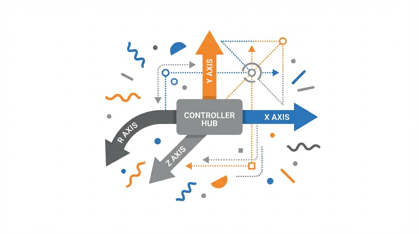
Four‑axis systems show up as SCARA manipulators, gantries, and XYZR positioning stages. Standard Bots describes 4‑axis arms with up/down, left/right, forward/back, and a rotation axis that give a near‑hemispherical workspace and payloads ranging from a few pounds to well over 40 lb for many industrial models, and even higher for heavy palletizing systems. Optimal Engineering Systems’ XYZR stages combine three linear axes with a rotary stage, with travels from roughly 0.6 in to almost 4 in and continuous 360° rotation, built on crossed‑roller bearings for rigid, smooth motion.

These platforms are ideal for complex but repeatable trajectories: intricate pick‑and‑place, packaging, laser processing, inspection, or logo machining. The limiting factor is rarely the mechanics. It is almost always the motion controller and the way trajectories are planned, executed, and tuned.

In this article I will walk through how to think about a 4‑axis motion controller for complex trajectories, leaning on published work from sources such as Automate.org, MDPI, ISA, Standard Bots, and others, and on what has worked repeatedly in real plants.

What A 4‑Axis Motion System Really Is

A 4‑axis system is not just “four motors.” It is four coordinated degrees of freedom that the controller must keep in lockstep.

Standard Bots frames a 4‑axis robot as an articulated arm with four joints that produce up/down, left/right, forward/back, and rotation motion via a manipulator, end‑effector, drive train, controller, and power supply. Sensors and sometimes machine vision feed joint position and motion back to the controller so it can execute smooth, repeatable movements.

The XYZR stages described by Optimal Engineering Systems are another concrete example. They provide X, Y, and Z linear motion on lead screws with fine pitch, plus an R axis with a 2.4 or 3.9 in rotary table. They are offered with stepper motors or closed‑loop servos with encoders, and they add limit switches and home switches so the motion controller can reliably home and protect the mechanics.

On the educational and light‑industrial end, Elephant Robotics’ 4‑axis myPalletizer arm and other similar platforms use a mainstream palletizing structure. They trade orientation flexibility for speed and simplicity, and they are explicitly positioned as stepping stones to full industrial robots while still supporting topics such as Denavit–Hartenberg kinematics, inverse kinematics, and machine vision.

From a motion‑control perspective, all of these share the same challenge: the controller must coordinate four axes in space and time so that the tool tip follows a planned trajectory, within error bounds, under real loads.

Motion Controller Fundamentals You Cannot Skip

Electromate and Automate.org both describe motion controllers as the “brain” of the system. They accept desired motion in various forms, plan trajectories in real time, and output synchronized signals to drives across multiple axes.

Several fundamentals matter for 4‑axis complex trajectories.

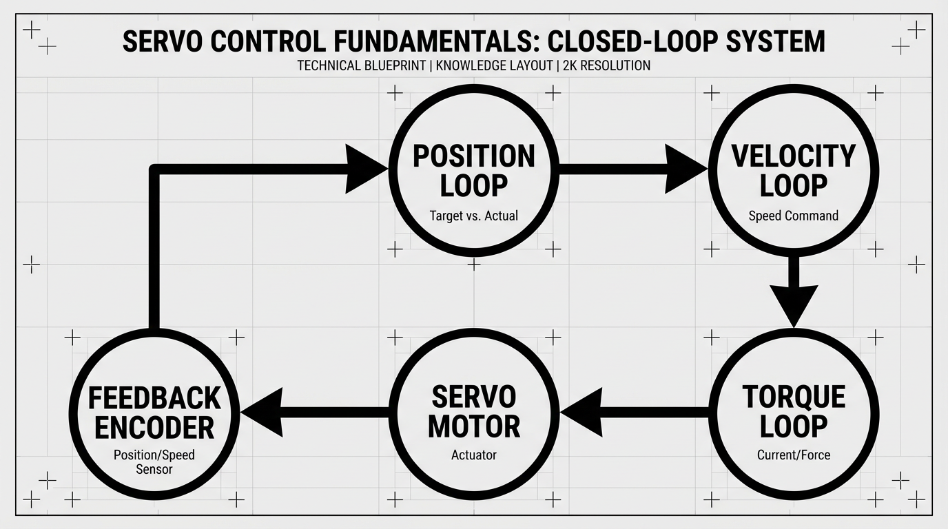
First, closed‑loop servo behavior. ISA explains that modern servo systems wrap position, velocity, and current (torque) loops together. The outer position loop computes position error and commands a velocity; the velocity loop in turn commands a current loop to change torque. Servo tuning is the art of adjusting gains in these loops so the axis responds quickly but without overshoot or oscillation.

Second, feedback quality. Motion‑control primers from Automate.org and Rexel highlight encoders as the primary feedback element, with quadrature encoders providing incremental position and direction, and absolute encoders and resolvers providing absolute position. High‑resolution feedback, with encoders reaching tens of millions of pulses per revolution, feeds smarter drives that can suppress vibration and execute fine trajectories.

Third, closed‑loop discipline. Following error—the difference between commanded and actual position—is both a key diagnostic and a common fault. ISA notes that if gains are too high, axes whine, draw excess current, and may overheat; if gains are too low, they may never settle properly and will fault on excess following error. Many “trajectory problems” are in fact servo‑loop problems.

Finally, multi‑axis coordination. Solo Motor Controllers defines multi‑axis motor control as simultaneous, coordinated control of two or more motors, where each axis represents a degree of motion and the controller must calculate and adjust position, speed, and torque in real time for every axis. This is fundamentally harder than single‑axis motion, because the controller must preserve global accuracy and balance while respecting limits for each individual axis.

If your 4‑axis motion controller cannot do these basics robustly—accurate feedback, well‑tuned servo loops, tight following error, and real multi‑axis coordination—no amount of trajectory sophistication will rescue the system.

From Path To Trajectory On Four Axes

One of the most useful distinctions in the MathWorks trajectory‑planning guidance is between path and trajectory.

They define task planning as choosing high‑level goals, path planning as defining a feasible geometric path as a sequence of waypoints, trajectory planning as assigning a time schedule for how to follow that path under position, velocity, and acceleration constraints, and trajectory following as the control system that executes that time‑parameterized path.

For complex 4‑axis systems, all four layers matter, but the handoff between path planning and trajectory planning is where many designs go wrong.

Task Space Versus Joint Space

MathWorks distinguishes task‑space trajectories, defined on the Cartesian pose of the end effector, from joint‑space trajectories, defined directly in joint coordinates. Task‑space trajectories usually look more “natural” and handle obstacles better, but they require frequent inverse‑kinematics solves, which can be computationally expensive. Joint‑space trajectories are cheaper to compute and can give very smooth actuator motion, but they do not guarantee obstacle avoidance or even adherence to joint limits at intermediate points.

The MDPI paper on a vision‑guided 4‑axis arm takes the classical route: full kinematic analysis via the Denavit–Hartenberg model, forward and inverse kinematics, and then trajectory planning in both joint and Cartesian space. They even use a Monte Carlo method with ten thousand random joint configurations to confirm that the 4‑axis arm’s workspace actually covers the desired task region. That kind of sober kinematic sanity check is worth copying.

In practice, for 4‑axis systems that run repetitive paths, I see a hybrid approach succeed most often: plan Cartesian paths in an offline tool where inverse kinematics and collision checks are available, then convert them into joint‑space trajectories with explicit limits and smoothness constraints for the controller.

Trajectory Profiles: Trapezoids, Polynomials, And Splines

The MathWorks example walks through the classic trajectory types your controller should support.

Trapezoidal‑velocity trajectories use piecewise constant acceleration, then zero acceleration, then constant deceleration. They produce a trapezoidal velocity profile and a linear‑segment‑with‑parabolic‑blend position profile. They are easy to implement and tune directly to position, speed, and acceleration limits.

The ODrive community has an implementation of a trapezoidal planner integrated into their servo firmware. Their planner computes a trajectory every control cycle and feeds position and velocity setpoints to the inner loops, handling corner cases like short moves and mid‑move limit changes. The algorithm is designed for extension to jerk‑limited profiles and to multi‑axis synchronization by computing time‑optimal trajectories per axis and then re‑planning all axes for the slowest time. Those ideas translate directly to 4‑axis industrial controllers.

Polynomial trajectories, such as cubic and quintic polynomials between waypoints, give smoother acceleration than trapezoids, but are harder to validate because constraints are encoded indirectly via boundary conditions. MathWorks notes that cubic polynomials require position and velocity at both ends; quintic polynomials require position, velocity, and acceleration. They are especially useful for stitching segments while controlling acceleration at joints.

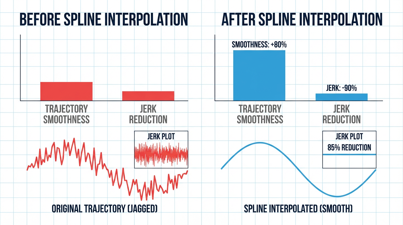
Spline‑based trajectories, including B‑splines, build complex shapes from piecewise polynomials. A B‑spline is controlled by points whose convex hull bounds the path, which makes it easier to shape motion without overshooting constraints. The MDPI work on “Optimal Trajectory Planning for Manipulators with Efficiency and Smoothness Constraint” uses quintic B‑splines in joint space to ensure that position, velocity, acceleration, and jerk are all continuous and smooth.

For a 6‑DoF manipulator drawing the Zhejiang University logo—a complex path of many discontinuous closed segments—they use cubic interpolation in Cartesian space, then map to joint space and apply fifth‑order B‑spline interpolation. They report that standard deviations of joint acceleration and jerk drop by more than 90 percent for most joints after interpolation compared with direct inverse‑kinematics profiles. That is a strong argument for using spline‑based smoothing in any 4‑axis system that has to follow complex trajectories without shaking the mechanics apart.

Handling Corners, Small Segments, And High Speeds

Real industrial paths are rarely single smooth curves. They are often built from many small linear segments: contouring around a part, machining a logo, or following a scanned profile. Without careful planning, these corners become speed killers and sources of vibration.

The real‑time look‑ahead trajectory‑planning work in a machining context shows a practical way forward. The authors insert quintic Bezier curves between small line segments to turn a polyline into a path with curvature continuity. They enforce G2 continuity—continuous position, tangent, and curvature—by constraining Bezier control points at the connections. Because quintic Bezier curves have enough degrees of freedom, they can match both tangent and curvature at the entry and exit of each segment.

They then compute curvature along the Bezier and derive a velocity limit at each point based on maximum normal acceleration and jerk. The velocity limit is set as the minimum of the limits from normal acceleration, jerk, and the global speed cap. The result is a look‑ahead planner that naturally slows down for tight corners with high curvature and accelerates in straighter sections.

Cornering error, defined as the distance between the midpoint of the transition curve and the intersection of the original line segments, is kept within a specified tolerance by adjusting Bezier parameters, so the smoothed path stays close to the original geometry.

Those exact techniques generalize nicely to a 4‑axis gantry or XYZR system.

If your trajectory is built from many small line segments, investing in quintic Bezier transitions or spline‑based smoothing with curvature‑aware feed‑rate limiting is usually worth more than yet another notch of controller bandwidth.

Efficiency Matters: Sequencing Complex Paths

Complex trajectories are not only geometrically demanding; they are also efficiency problems. The MDPI study on optimal trajectory planning uses the Zhejiang logo as a case study not just for smoothness, but for efficiency in moving between many discontinuous closed paths.

They model the centers of each closed contour as “cities” and use an improved ant colony optimization algorithm to find an order that minimizes non‑productive motion. They compare this to a genetic algorithm and particle swarm optimization under identical conditions.

Across multiple simulation runs, the improved ant colony method finds an average optimal free‑load path of about 1273 mm, while the genetic algorithm and particle swarm optimization produce about 2397 mm and 3280 mm respectively. Converted to imperial units, that is roughly 4.2 ft of non‑productive travel versus 7.9 ft and 10.8 ft.

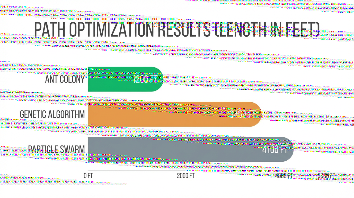
The improved ant colony method also converges in fewer iterations and shows lower variance between runs.

Once they have an efficient visiting order, they apply the Cartesian and joint‑space spline planning described earlier, and then validate experimentally on the robot, showing accurate and smooth reproduction of the logo.

For a 4‑axis system that has to visit many work locations—multiple pallets, nests, or part features—thinking of the problem as “sequence optimization plus smooth interpolation,” rather than just “follow these points in the order the CAD model happened to give them,” can unlock substantial throughput without touching the hardware.

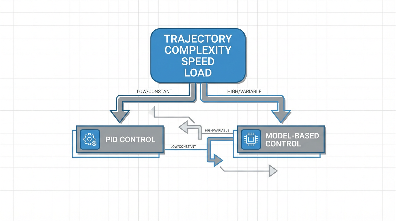
Control Strategy: PID Or Model‑Based On 4 Axes?

Trajectory planning is only half the story. The low‑level control strategy you deploy on each axis determines whether those trajectories are achievable in the real system.

A recent ScienceDirect study compares decentralized PID and model‑based computed torque control on an open PLC‑based controller driving a four‑degree‑of‑freedom SCARA manipulator. They frame the problem clearly.

PID controllers are simple, model‑free, and widely understood. In typical automation plants, PLCs control motors on conveyors and other equipment using independent PID loops on each axis. Applying that same pattern to robot joints is attractive: tuning tools already exist and commissioning teams are familiar with the behavior. Research cited in their paper suggests proprietary industrial robot controllers may also rely on PID at their core, although the details are usually undisclosed.

The downside is that decentralized PID treats each joint independently. It does not explicitly compensate for nonlinear dynamics, coupling between joints, or changing inertia as the arm moves. The result can be limited tracking performance on fast or curved trajectories, especially for tasks such as welding and laser cutting where path error directly affects product quality.

Model‑based controllers such as computed torque control, model predictive control, and adaptive control explicitly use the robot’s dynamic model. They compute control actions that include gravity, Coriolis, and inertial terms, and they treat the joints as a coupled system. The study notes that these methods can offer superior trajectory tracking, but they require accurate dynamic parameters and more computational effort, and that identifying those parameters can be complex and time‑consuming.

Open PLC‑based controllers add another dimension: control frequency. If you can raise the control loop frequency for a PID controller, how close can you get to the performance of a more complex model‑based algorithm at a lower frequency? The ScienceDirect paper is structured around precisely that question, along with the effect on PLC CPU load.

The authors set up a series of experiments comparing PID and computed torque control across different path geometries, velocity profiles, and PLC frequencies, and they quantify both tracking error and CPU load. While the detailed results are beyond the excerpt available here, the message for practitioners is clear: on a 4‑axis system, do not assume that PID at a high control rate will or will not match a model‑based scheme. Test it on representative trajectories, measure tracking error and CPU utilization, and choose based on data rather than habit.

How Four Axes Change The Trade‑Offs

Because a 4‑axis system has fewer joints than a 6‑axis arm, some of the complexity in dynamic coupling is reduced, but it does not disappear. Standard Bots points out that 4‑axis arms have less articulation than 6‑axis models, but often higher stability and carrying capacity, and they are well‑suited to flexible but straightforward pick‑and‑place, assembly, handling, inspection, and packaging tasks. For those applications, a carefully tuned PID controller on each axis, with reasonable feed‑forward and smooth trajectories, may be enough.

However, when you push 4‑axis systems into more demanding roles—complex machining patterns, high‑speed inspection with continuous orientation changes, or precise multi‑surface laser processing—the arguments for model‑based control begin to resemble those for 6‑axis robots. The MDPI work on the vision‑guided 4‑axis arm emphasizes full kinematic modeling and trajectory planning, and the ScienceDirect study underscores that open controllers give you the latitude to choose.

As a systems integrator, I usually start 4‑axis projects with robust PID control and high‑quality trajectories, and only move to model‑based control when measurements show that the combination of trajectory complexity, speed, and load pushes PID beyond its comfort zone.

Architecting The 4‑Axis Motion Platform

The architecture of the motion system—mechanism, motors, drives, controller, and HMI—sets the boundaries of what your trajectories can do.

Automate.org breaks a motion system into five major elements. The mechanism is the physical stage or arm. The motor converts electrical to mechanical power. The drive (or amplifier) powers and commutates the motor. The controller generates trajectories and setpoints. The HMI provides the operator interface.

Servo motion‑control basics from ISA and Electromate emphasize several practical design points. Motor and drive sizing must account for inertia, duty cycle, and required settling times; otherwise, tuning may be impossible. Environmental demands—sterilizable medical equipment, fluids, or sea water—drive choices around motor types and enclosures. Feedback devices must be chosen for both resolution and robustness.

The XYZR stages from Optimal Engineering Systems illustrate one sensible design pattern for 4‑axis platforms. Linear axes use fine‑pitch lead screws, high‑precision crossed‑roller bearings, and limit switches. The rotary axis has a home switch for zeroing and a through‑hole and mounting patterns to support tooling and cable routing. Motors can be stepper or servo, with or without encoders. The vendor can pair these with multi‑axis motion controllers for a plug‑and‑play stack.

At the controller level, Rexel and Electromate describe motion controllers that support multiple motion types—point‑to‑point moves, continuous constant‑speed motion, and synchronized multi‑axis motion. Modern controllers often integrate safety functions and can coordinate several dozen axes when plugged into a PLC backplane. Open networking standards such as EtherCAT and PLCopen motion function blocks make it possible to integrate multi‑vendor drives and feedback into a coherent system.

Multi‑axis motor control, as Solo Motor Controllers describes it, is inherently about coordination.

Every control cycle, the controller must calculate target position, speed, and torque for each axis, respecting their individual limits while keeping the tool on the planned 4‑D trajectory. That is true whether you are using an embedded motion controller, a PLC‑based open controller, or a PC‑based system.

A Practical Design And Commissioning Workflow

On paper, trajectory planning and control design can appear abstract. On the plant floor, they are a sequence of concrete decisions and tests. A practical workflow for a 4‑axis complex trajectory system usually looks like this.

First, clarify the task. Are you palletizing, machining, inspecting, packaging, or drawing complex paths? The MDPI cases on logo tracing and object grasping, and the Standard Bots discussion of 4‑axis applications in assembly and inspection, make it clear that the nature of the task drives path geometry, speed, and accuracy requirements.

Second, validate the kinematics. Follow the example of the MDPI 4‑axis arm study: build a proper kinematic model, run forward and inverse kinematics, and use Monte Carlo sampling or similar to ensure that the 4‑axis workspace actually covers your intended volume without singularities in the critical region.

Third, design and simulate trajectories. Use the MathWorks toolbox ideas as a template. Start with simple trapezoidal profiles and then explore polynomial or spline trajectories. For complex shapes or many small segments, consider quintic Bezier smoothing and curvature‑based feed‑rate limiting, as in the machining look‑ahead work, or joint‑space B‑splines, as in the MDPI smoothness study. Validate against position, velocity, acceleration, and jerk limits.

Fourth, decide on your low‑level control strategy. Think in the terms used by the PLC‑based study: is a decentralized PID controller, possibly with adaptive or nonlinear enhancements, sufficient at a given control frequency for the required trajectories? Or do you need model‑based computed torque control? Plan experiments to answer this, rather than assuming.

Fifth, tune the servo loops and verify following error. Apply the guidance from ISA and Rexel: adjust gains until axes respond crisply without oscillation; watch for excess following error alarms and for signs of mechanical interference. Do not blame the controller before you have ruled out mechanical issues.

Sixth, iterate using data. The TACO work on quadrotor trajectory‑aware controller optimization provides a useful mindset even for 4‑axis hardware. They build a predictive model of controller performance as a function of gains, current state, and upcoming trajectory segment, and then use it online to adapt gains and even adjust the trajectory itself to improve dynamic feasibility. You do not need a neural network on a 4‑axis palletizer, but you should certainly log tracking error, CPU load, and fault history, and use that data to refine gains and trajectories over time.

Finally, confirm everything in real production conditions, not just in a test cell. The MDPI logo experiments and the 4‑axis vision‑guided arm trials both emphasize that simulation and lab validation are starting points, not endpoints. Real‑world loads, temperatures, and operators will reveal details that no model anticipated.

Common Mistakes I See With 4‑Axis Controllers

Certain problems repeat across plants and industries.

One recurring mistake is treating the 4‑axis system as “just four single axes” and ignoring multi‑axis coordination. Solo Motor Controllers’ definition of multi‑axis control underscores that every axis must be computed together in real time. If you bolt four single‑axis drives to a PLC and issue independent profiles without a proper multi‑axis planner, do not be surprised when the tool path is distorted.

Another is underestimating jerk and curvature. The machining look‑ahead research and the MDPI smoothness study show that acceleration and jerk continuity matter greatly for vibration. Rough corners and piecewise‑constant acceleration trajectories can excite the mechanics, increase following error, and shorten component life.

A third is overcomplicating the control algorithm before fixing mechanical or trajectory issues. The ISA servo basics article notes that many following‑error faults are caused by mechanical interference or poor tuning, not by some lack of advanced control. If a 4‑axis gantry is binding in a corner or driven by an undersized motor, computed torque control is not a cure.

Finally, there is a procedural mistake: not giving technicians and engineers enough visibility. Modern controllers and drives can report following error, CPU load, vibration estimates, and even predictive maintenance diagnostics, as noted in articles from ISA and Electromate. Hiding that behind opaque HMIs or proprietary diagnostics makes troubleshooting harder than it needs to be.

Short FAQ

Do I really need a 6‑axis robot for complex trajectories?

Not always. Standard Bots points out that 4‑axis robots already offer higher dexterity than simple 3‑axis systems and cover a near‑hemispherical workspace, with payloads commonly in the 22 to 44 lb range and sometimes up to around 1,100 lb in palletizing configurations. If your trajectories live in a plane or a simple volume and do not require arbitrary orientation of the tool, a 4‑axis arm or XYZR stage, paired with a capable motion controller and the trajectory techniques discussed here, is often the most pragmatic choice.

Should I base my 4‑axis controller on a PLC or a dedicated motion controller?

The motion‑controller introduction from Electromate and the PLC‑based study in ScienceDirect both highlight viable paths. PLC‑based open controllers offer reliability, familiar programming environments, and emerging robot control libraries from major vendors. Dedicated motion controllers often provide higher‑end multi‑axis features and built‑in profiles. If you already have strong PLC expertise and need tight integration with other plant equipment, a PLC with an open motion library can be a solid foundation. If your trajectories are extremely demanding or your team lives in motion‑control toolchains, a dedicated controller may be better.

How do I know if my trajectories are too aggressive?

Servo‑motion articles from ISA and the trajectory‑planning research in MDPI give two perspectives. From the servo side, watch following error, overshoot, whining sounds, and drive temperatures; persistent following errors or oscillations at specific path features often signal that acceleration or jerk is too high. From the trajectory side, compute curvature and apply explicit acceleration and jerk limits, as the machining look‑ahead method does. If the planner must constantly clamp velocity to stay within dynamic limits, you either need softer paths or more capable mechanics and actuators.

Closing Thoughts

Four‑axis motion controllers sit at a very productive intersection of capability and practicality. With solid kinematics, curvature‑aware trajectory planning, disciplined servo tuning, and an honest choice between PID and model‑based control, a 4‑axis system can execute surprisingly complex trajectories day in and day out. In my experience, the teams that succeed treat trajectory planning and control as an integrated problem, measure everything they can, and choose the simplest architecture that still respects the physics. If you approach your next 4‑axis project that way, you will be a dependable partner to your operations team instead of the person they call only when the gantry is faulted at 2:00 AM.

References

1. http://manipulation.csail.mit.edu/trajectories.html
2. https://arxiv.org/html/2511.02060v1
3. https://www.automate.org/motion-control/industry-insights/understanding-motion-control-basics
4. https://www.isa.org/intech-home/2020/november-december-2020/departments/servo-motion-control-basics
5. https://www.researchgate.net/figure/Overview-of-the-proposed-four-axis-tool-path-generation-method_fig3_274419847
6. https://www.limonrobot.com/how-to-design-a-multi-axis-system-for-your-application
7. https://library.automationdirect.com/what-is-motion-control/
8. https://www.instructables.com/Simple-3-Button-Controller-for-a-4-Axis-Robot-Arm/
9. https://www.linearmotiontips.com/four-axis-positioning-stages-with-four-motor-options/
10. https://standardbots.com/blog/what-is-a-4-axis-robot