Fast Response Digital Output for Time-Critical Control Applications

When you chase microsecond response in an industrial system, the digital output channel is where theory meets the plant floor. Over the years integrating motion systems, robotics, and high-speed machinery, I have learned that fast digital outputs are rarely just about a “faster card.” They are about building a deterministic chain from sensor to silicon to field wiring to actuator, and making sure that chain keeps its promises every single scan.

This article walks through how to think about fast-response digital outputs in time-critical control applications, using the perspective of a systems integrator who has had to make these designs start, stop, and keep running in real factories. The discussion is grounded in published guidance from AOP Technologies on analog versus digital control, Control.com and Contec on digital I/O practice, application notes from Analog Devices and Monolithic Power, real-time control material from Texas Instruments, and practical closed-loop design work described by Vitrek and real-time DSP lectures in academia.

Digital Outputs In Real-Time Control: What They Actually Do

In industrial control, a digital output is a discrete, usually binary, signal used to drive something in the real world. Control.com emphasizes that in PLCs these outputs energize solenoid valves, motor starters, relays, contactors, pneumatic cylinders, lamps, and alarms. The underlying signals are 0 or 1, off or on, which maps naturally onto the way computers and microcontrollers operate.

Digital output modules sit between low-voltage logic and field-level devices. Contec describes several common circuit styles: non-isolated TTL or LVTTL for short, low-noise wiring; photocoupler-isolated transistor outputs for 12–48 VDC loads; and relay contact outputs when AC or high-voltage DC devices must be switched directly. In all cases, the digital output module has to translate a logic-level request from a controller into a clean transition in the field, with the correct polarity (sink or source), voltage, and current.

Control.com notes that digital outputs are preferred for many industrial tasks because they are fast and precise, scalable to many points per PLC, and robust when properly protected. Combined with relays or contactors, they can switch large motors, pumps, and heaters while keeping the logic electronics isolated from harsh electrical environments.

From a real-time control standpoint, a digital output is the last link in a closed loop.

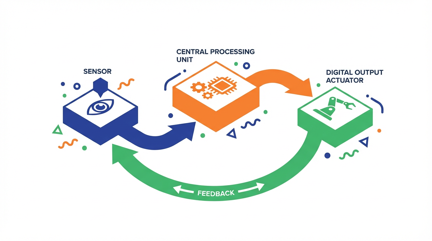
It must change state within a fixed timing budget that also includes sensing and computation. Texas Instruments defines real-time control as the ability of a closed-loop system to sense, process, and update outputs within a fixed time window; missing that window degrades stability, precision, and efficiency. In high-performance motor drives and robotics, these windows are often measured in microseconds.

How Fast Response Is Defined In Control Systems

Monolithic Power describes response time using classic control terms: delay time to reach roughly half the final value after a step, rise time between about 10% and 90% of the final value, peak time to the maximum overshoot, and settling time until the output stays within a small band of the target value. These definitions are usually applied to analog variables like position, speed, or voltage, but the same concepts apply around digital outputs.

For a discrete actuator driven by a digital output, you can think of several nested response times. There is propagation delay inside the driver from logic-level command to high-voltage output. There is the actuator’s own rise and settling time (a solenoid, a relay, a motor coil). And there is the closed-loop response of the larger system: how long it takes the controlled variable to settle after the output drives a step.

Real-time control material from Texas Instruments and WPI’s real-time DSP lectures emphasize another set of timing concepts: sampling period, computation time, and jitter. In a sampled-data control loop running at a fixed rate, the sampling period is the time between consecutive control updates. Computation time is how long the processor spends per update. Jitter is the variation in that period from one cycle to the next. In hard real-time applications, such as high-speed signal processing at 32 kHz or fast current loops in motor drives, the computation must finish strictly before the next sample, and jitter must be tightly controlled.

Vitrek’s work on a digital PID loop for sub-micron motion control adds a practical nuance: loop cycle processing time and jitter together determine how repeatable the loop timing really is. In their implementation, a 500 microsecond control cycle is used, and the variation of that cycle from one iteration to the next is explicitly defined as jitter. They show that a faster theoretical loop time, such as 200 microseconds, can produce better modeling resolution but worse jitter, which may hurt overall performance.

In short, “fast response digital output” is not just a fast edge. It is the ability to produce that edge at precisely the right time, and to do so continuously over many cycles without missing deadlines or accumulating jitter that undermines stability.

Digital Versus Analog Paths For Time-Critical Actuation

AOP Technologies compares digital and analog control in proportional measurement and automation systems. Analog control has important advantages: it processes signals continuously, often with very low intrinsic latency, and can be simple and cost-effective for basic loops. In applications where smooth, uninterrupted response is critical, such as certain proportional valve controls, analog electronics still shine.

The same article highlights analog drawbacks that matter in harsh industrial environments: susceptibility to noise and electromagnetic interference, component drift that requires frequent calibration, and limited flexibility because changes usually require hardware modifications. That is a non-starter in many modern plants that expect recipe-driven changeovers and remote diagnostics.

Digital control, by contrast, implements algorithms on microcontrollers, DSPs, or FPGAs. Monolithic Power notes that digital controllers can implement sophisticated algorithms such as predictive or adaptive control, and Tiverts that they enable integrated data logging, analytics, and network connectivity. AOP Technologies and Monolithic Power both emphasize that digital systems are more immune to noise and easier to reconfigure through software.

The price of this flexibility is potential latency and sampling effects. Sensors often output analog signals that must be sampled and quantized; the controller then computes a result, and only then can a digital output be updated. AOP Technologies points out that A/D conversion and computation time can introduce latency, and that digital systems are dependent on a stable power supply and careful timing design.

When you care about fast digital outputs, the practical balance is as follows. If your loop absolutely cannot tolerate any sampling or computation delay, a simple analog path may still be best. If you need complex logic, tight integration with the rest of an Industry 4.0 architecture, and robust operation over time, a digital path with carefully designed timing is the practical answer. Most real systems land in the middle: analog front-ends and drivers with a digital controller orchestrating behavior.

Hardware Building Blocks Of A Fast Digital Output Path

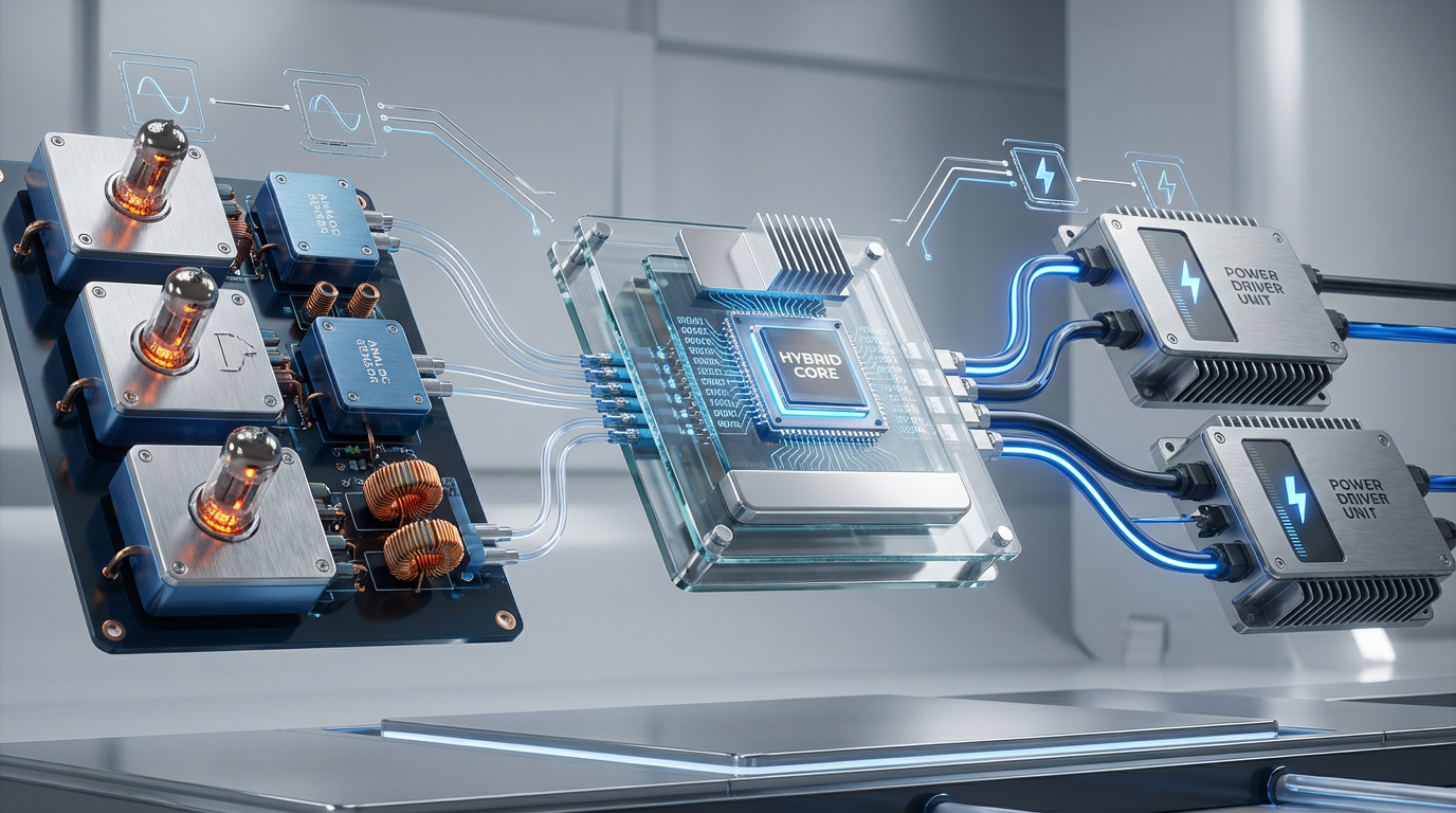
A fast digital output chain is only as quick as its slowest element. Monolithic Power’s introduction to digital control systems in power electronics describes the typical architecture: sensors feeding ADCs, a digital controller running control algorithms, DACs or direct digital drive of power devices, and actuators driven via feedback loops. Contec’s digital I/O guidance and Analog Devices’ design note on digital output drivers add detail on the output side.

At the controller level, Texas Instruments notes that real-time control MCUs such as C2000 devices can execute fast loops in the microsecond range, with integrated analog peripherals to reduce external latency. More complex systems, such as those described by Vitrek, may use embedded x86-class platforms running a real-time operating system and interacting with digital sensors over Ethernet. Boston Engineering’s discussion of embedded real-time systems describes the role of microcontrollers, FPGAs, and RTOS platforms in delivering deterministic real-time behavior for robotics, medical devices, and other demanding applications.

The digital output driver is the bridge between logic and the 12–36 V world. Contec describes non-isolated TTL outputs for short-distance logic-level interfacing; photocoupler-isolated transistor outputs that can sink or source DC loads from about 12 to 48 V; and relay contact outputs that can switch AC or higher-voltage DC at the cost of slower switching speed. Transistor outputs are available in sink-compatible configurations, where current flows from the load into the output, and source-compatible configurations, where current flows from the output into the load. This sink/source distinction matters for matching what your field devices expect.

Analog Devices’ design note on digital output drivers uses octal high-voltage drivers such as the MAX14912/MAX14913 as examples. These integrate eight channels, operate from about 12 to 36 V, tolerate power spikes up to 60 V, handle ±1 kV surge pulses and up to 12 kV ESD, and can switch at frequencies up to roughly 200 kHz. They are specified over a wide temperature range, from around –40°F up to approximately 257°F, making them suitable for industrial cabinets and field boxes. On-chip features include a 5 V DC-DC converter that can supply more than 100 mA to external logic, and the ability to parallel high-side outputs so that several channels can jointly drive loads up to about 9.6 A.

Digital output drivers must also match the controller interface. Analog Devices explains that these parts can be controlled via simple parallel inputs using several GPIOs or via a serial SPI interface. The parallel interface offers minimal protocol overhead and can be attractive for latency-sensitive outputs, but it requires more pins. SPI enables richer configuration and diagnostics through internal registers, at the price of serial transfers that consume time on each update.

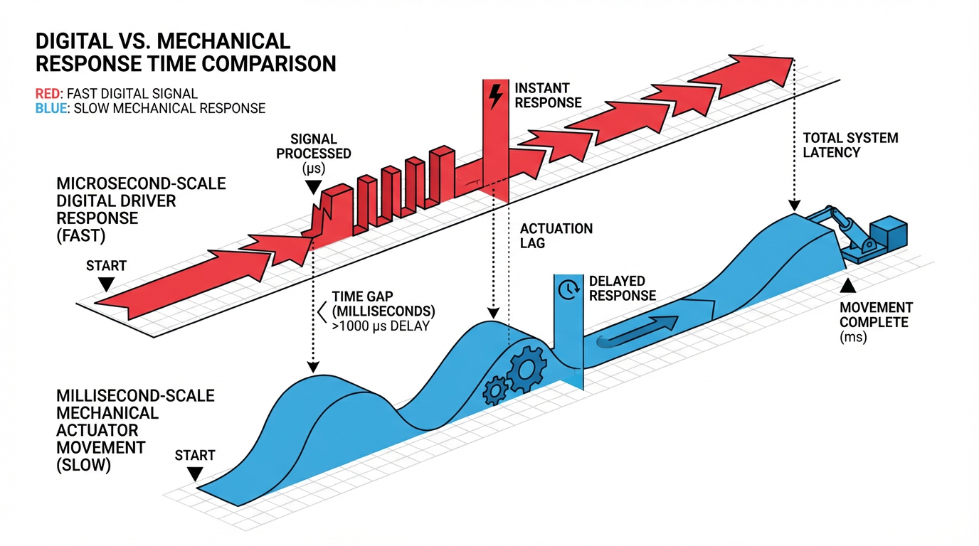
Finally, there is the load and field wiring. Control.com notes that digital outputs in PLCs often feed relays if the final load is a motor or heater. Contec describes that DC transistor outputs are well suited for 12–48 V loads such as indicator lamps, small DC actuators, and relay coils. Relay contact outputs can handle AC and strong DC loads above 48 V but are mechanically limited in speed. From a fast-response standpoint, it is easy to obsess over microseconds in the driver while the actual bottleneck is a relay armature or a mechanical solenoid that moves in milliseconds. A realistic design has to consider both.

Latency And Jitter: Where Digital Outputs Really Lose Time

Real-time DSP lectures from WPI categorize many fast signal-processing applications as hard real-time problems. An example used there is continuous audio processing at 32 kHz. If a new sample is not ready exactly when the DAC needs it, even by about a microsecond, the effective sampling rate is disturbed and audible distortion appears. That lecture carefully breaks down the sample period into input, processing, and output work, and defines slack as the difference between the total sample period and the time actually spent computing. Processor load is then the ratio of computation time to sample period.

An important observation from those lectures is that a surprisingly large fraction of the cycle can be consumed by ADC and DAC handling rather than the actual signal-processing algorithm. In one example, a polled I/O implementation using an MSP432 microcontroller and a 14-bit DAC achieves a sample period of around 17 microseconds, about 55.8 kHz, at a 48 MHz CPU clock. That corresponds to roughly 800 clock cycles per sample. Only about 50 cycles are actually spent on the user processing function, while about 750 cycles are consumed by ADC conversion, interrupt latency, and DAC update, including roughly 273 cycles spent simply asserting and de-asserting a GPIO-driven SYNC signal and moving two bytes over SPI to the DAC.

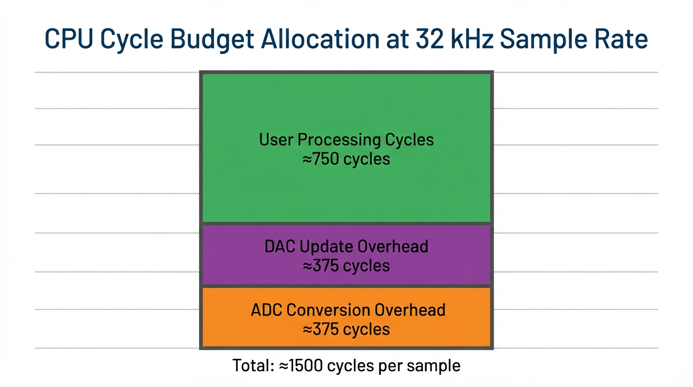
The implications for digital outputs are straightforward. Even if the driver chip can toggle at 200 kHz, the combination of bus protocol, housekeeping code, and the rest of the loop may reduce the effective update rate by an order of magnitude. At moderate sample rates, such as 8 kHz, the WPI material estimates that about 6,000 cycles are available per sample at 48 MHz, but about 750 of those cycles are consumed by basic ADC and DAC management, leaving only about 5,250 cycles for the core algorithm. At higher sample rates, for example around 32 kHz, the total budget becomes about 1,500 cycles per sample, so that same fixed overhead now eats half the budget, leaving about 750 cycles for user processing.

Software structure strongly affects how predictable this timing is. The WPI lectures compare a fully polled I/O loop against a timer-driven interrupt scheme. In a polled loop, each iteration triggers an ADC conversion, waits for it to finish, reads the sample, processes it, and then drives the DAC. The sampling rate is determined by how long the whole loop takes, which in turn depends on the complexity of the code. This can be acceptable when the code has constant execution time and sample rate tolerances are wide, but it is fragile for time-critical control.

In a timer-driven approach, a periodic hardware timer triggers ADC conversions at precise intervals. At the end of conversion, the ADC raises an interrupt, whose service routine reads the sample, runs the processing function, and updates the DAC. The main loop mostly sleeps. As long as the interrupt handler finishes before the next timer event and its execution time is effectively constant, this gives a highly deterministic sample rate. The WPI lectures recommend monitoring the DAC’s SYNC pulse on a scope and checking that its frequency matches the intended sample rate. If the measured frequency is lower, it indicates that some interrupts are being missed and that the system is no longer truly real-time.

Vitrek’s motion-control example illustrates the same timing concerns in a different context. Their digital closed-loop system uses a capacitance sensor (MTI Digital Accumeasure) for sub-micron displacement feedback and a piezo stage with about 100 micrometers of travel, roughly 0.004 inches. The controller is an embedded Intel Atom platform running a real-time operating system, with all I/O handled digitally. The motion control software is organized into tasks that handle Ethernet communication with the sensor, make the process variable data available, and run a PID loop. The control loop executes every 500 microseconds.

Their analysis shows that sensor and communication latency matter at least as much as the controller’s own loop speed. With the sensor filter set for its highest bandwidth, the Digital Accumeasure contributes about 2.14 milliseconds of latency, and Ethernet communication adds around 800 microseconds per packet. The piezo stage’s own mechanical dynamics contribute on the order of 10 milliseconds. Even though the control loop runs every 500 microseconds, the overall closed-loop response is around 50 milliseconds, determined by the sum of these delays and the multi-cycle nature of the PID controller.

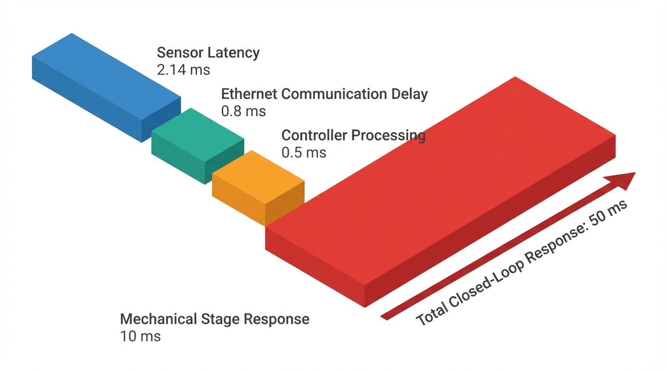
They also show that a shorter nominal loop period of 200 microseconds offers finer sampling of the stage’s time constant, but with more jitter, making the 500 microsecond period a better practical choice.

From these examples, a pattern emerges. In digital control systems, fast digital outputs are necessary but rarely sufficient. The latency and jitter budget is shared across ADCs, computation, communication buses such as SPI or Ethernet, and the physical actuator. A design that only optimizes the digital output switching speed but ignores these other pieces will not deliver the fast, stable response that time-critical applications demand.

Output Driver Design For Fast Response

On the output side, driver topology and configuration have a direct impact on achievable response and robustness. Analog Devices explains two main modes of operation in their MAX14912/MAX14913 digital output drivers: push-pull and high-side. In push-pull mode, each channel actively drives both high and low states. This yields fast, sharp waveforms and is well suited to high-speed communication signals or loads that require tight edge control. In high-side mode, the driver can present a high-impedance state and allows outputs to be paralleled, which is valuable for driving higher currents, but the exact timing and waveform shape depend more on the load and its impedance.

Contec details additional choices in digital I/O circuits. Photocoupler-isolated transistor outputs provide galvanic isolation and good noise immunity, but the photocoupler introduces propagation delay and limits maximum switching speed. Non-isolated TTL or LVTTL outputs avoid that delay and can toggle very quickly, but should be used only where wiring distances are short and noise is controlled. Relay contact outputs can switch both AC and DC loads, including strong loads above about 48 VDC, but mechanical contacts are much slower and unsuitable for very fast response.

If you are designing for fast response, the tradeoffs look like this. Non-isolated TTL outputs have the smallest intrinsic delay and can respond at high rates, but they are fragile with respect to noise, ground potential differences, and field-level transients. Photocoupler-isolated transistor outputs offer good speed for 12–48 VDC actuators while providing isolation and noise immunity; the propagation delay is usually negligible compared with mechanical actuation times, but it is not zero. Relay outputs are naturally limited by millisecond-scale contact movement and are best reserved for slow or infrequent switching.

The Analog Devices design note also stresses system integration features that support reliable fast operation. Their drivers interface low-voltage logic levels, from around 1.6 to 5.5 V, to 12–36 V actuators while providing protection and diagnostics. They include detection of open-load conditions, under-voltage and over-voltage events, overcurrent and overtemperature shutdown, and per-channel fault reporting via status registers. A 4-by-4 LED crossbar can be used on a panel to visualize output state and faults without external wiring, which is helpful during commissioning and troubleshooting.

Control interfaces matter as well. Analog Devices describes a parallel control mode that uses at least nine GPIOs for eight channels plus a mode pin and provides minimal diagnostics, and a serial SPI mode that enables full configuration and detailed fault reporting through internal registers. Direct SPI modes allow the controller to set outputs directly with eight or sixteen-bit words, while command modes use a command byte plus a data byte to access configuration and diagnostic registers. They recommend configuring mode and protection registers first, then updating output levels, to avoid surprises.

Because high-speed SPI transactions consume CPU time and bus bandwidth, designers must weigh how often they need to toggle an output and how much diagnostic information they need. For a few channels that must switch extremely quickly, a simple parallel interface can make sense.

For large banks of outputs in a PLC-like node, SPI with daisy-chained drivers, as described in the Analog Devices note, scales well and enables rich diagnostics, even if individual outputs cannot be updated at hundreds of kilohertz.

Finally, protection and communication integrity features need to be considered in the timing budget. Analog Devices describes an optional seven-bit CRC scheme for SPI commands using a specific polynomial. When enabled, each SPI command includes a CRC check byte. If the received CRC does not match, the command is ignored and a fault bit is set. This improves reliability in noisy industrial environments but adds a few bits to every SPI transaction and requires the controller to compute the CRC, which adds a small amount of latency. Similarly, watchdog timers that detect loss of communication and global fault handling logic must be configured thoughtfully so that protective actions do not inadvertently slow or block time-critical updates.

System-Level Practices For Fast And Reliable Digital Outputs

Fast digital outputs make sense only in the context of the system they serve. Several of the sources emphasize starting from application requirements rather than from component data sheets.

First, derive timing requirements from the process and stability needs. Monolithic Power explains that aggressive tuning for fast response can reduce settling time but risks overshoot, oscillation, and instability. Slower but well-damped responses are often acceptable in processes such as climate control, where thermal inertia is high, but in high-speed motion control or power electronics, timing windows are tight. Texas Instruments discusses robot arms achieving position accuracy better than 100 micrometers, roughly 0.004 inches, and high-precision CNC equipment reaching accuracy better than about 5 micrometers, approximately 0.0002 inches, at rotational speeds exceeding 20,000 rpm. Those applications require measurement-to-adjustment delays below one microsecond in some control loops. That level of performance should drive your sampling rates, computation budgets, and digital output specifications.

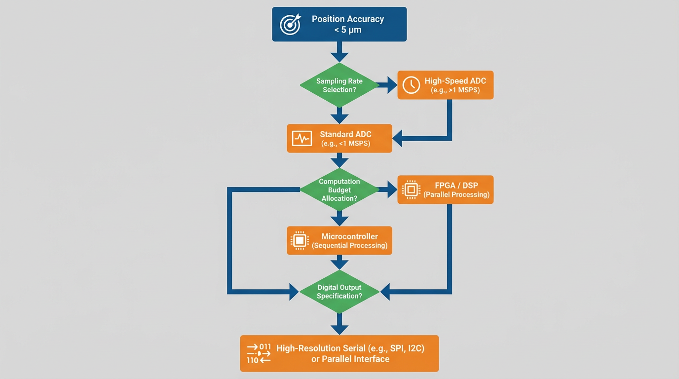
Second, architect the real-time loop so that the digital output is not the bottleneck. Texas Instruments and Boston Engineering both describe real-time control systems as a chain of sensing, control processing, and actuation, with deterministic communication between elements. Where loops must be extremely fast, TI notes that FPGAs, fast external ADCs, and multiple MCUs are often combined. In other cases, TI highlights that high-integration MCUs can implement current-loop execution under one microsecond on a single chip. For motion systems like the one in Vitrek’s work, an RTOS provides scheduling guarantees for different tasks, but the designer still needs to choose a loop cycle time that balances modeling fidelity, jitter, and overall latency.

Third, specify digital output hardware with a clear view of field devices and wiring. Contec recommends choosing the number of outputs based on the number of relays or loads, with additional outputs reserved for alarms, reset signals, and handshakes. They provide similar guidance for digital inputs used to monitor switches. Their material also reminds designers that logic conventions differ: many isolated DC inputs use positive logic, where an ON or closed contact is logic 1, while some TTL-level circuits use negative logic, where a low level represents logic 1. Getting that wrong at the specification stage leads directly to field rewiring and lost time.

Fourth, implement deterministic software. The WPI real-time DSP lectures recommend minimizing data-dependent branches and loops in per-sample code, to keep execution time constant. Timer-driven ADC triggers and interrupt-driven processing, rather than polling loops, give more predictable sampling. Simple techniques such as toggling a debug pin around a processing function and observing its duty cycle on an oscilloscope, as described in those lectures, provide hard evidence of how much time each function consumes and whether it fits in the sampling window.

Fifth, validate the entire digital output path with measurement. Vitrek’s work shows the value of breaking down latency between sensor, communication, controller, and actuator, rather than treating the loop as a black box. Their analysis of the Digital Accumeasure latency, Ethernet delay, and piezo stage dynamics leads to a realistic understanding of why the overall closed-loop response is about 50 milliseconds, even with a 500 microsecond update period. In a similar way, WPI’s approach to monitoring DAC SYNC frequency directly reveals whether samples are being dropped. For digital outputs controlling actuators, you can monitor both the logic-level output and the actual actuator current or position to see where time is being lost.

Pros And Cons Of Pushing Digital Outputs To The Limit

It is natural to assume that faster is always better. The literature paints a more nuanced picture.

On the benefit side, Monolithic Power explains that faster response reduces delay, rise time, and settling time between setpoint and process variable. Texas Instruments shows that in motor drives and robotics, sub-microsecond current and position loops enable high accuracy, high speed, and better efficiency, especially when combined with advanced power devices such as GaN FETs. Vitrek’s motion-control experiments demonstrate that carefully tuned digital PID control with a well-chosen loop period can deliver closed-loop settling times around 50 milliseconds, significantly faster than more conservative tuning, without overshoot.

On the drawback side, Monolithic Power warns that overly aggressive tuning or insufficient damping leads to oscillations and potential instability. Their discussion of stability analysis using Bode plots, Nyquist criteria, root locus, and Routh–Hurwitz underscores that closed-loop poles must stay in stable regions. Faster responses can also increase power consumption and thermal stress, particularly in high-sampling-rate digital control and power electronics, where rapid changes in actuator signals translate to switching losses and heating. Vitrek’s comparison between “moderate” and “aggressive” tuning shows that aggressively fast PI control can produce overshoot and oscillations that are unacceptable in precision motion systems, even if the numeric settling time is shorter.

There is also a reliability dimension. Analog Devices describes how digital output drivers have to survive ±1 kV surge events and 12 kV ESD, while operating over a wide industrial temperature range. Running outputs at very high switching frequencies and edge rates increases electromagnetic emissions and can stress both the driver and the load. Design features such as integrated diagnostics, overcurrent protection, and CRC-protected SPI communication exist precisely because industrial environments are electrically noisy. It is often better to operate slightly below theoretical maximum speed while ensuring robust protection and error detection, than to run at the edge and invite intermittent faults.

A pragmatic approach, and one that aligns with both the published guidance and practical project experience, is to push speed only as far as the process and stability margins truly demand, and then spend at least as much effort on determinism, robustness, and diagnostics as on raw edge rate.

Brief FAQ

Do I really need microsecond-level digital outputs for my application?

According to Texas Instruments, only certain classes of systems, such as high-precision CNC machines with accuracy better than about 5 micrometers at speeds above 20,000 rpm or advanced robotic arms targeting better than roughly 100 micrometers, require measurement-to-adjustment delays below one microsecond. Most temperature, pressure, and slow mechanical processes can tolerate much slower response. AOP Technologies and Monolithic Power both encourage designers to start from required precision, environmental conditions, and flexibility rather than chasing digital performance numbers that the process does not need.

When should I prioritize isolation and protection over raw output speed?

Contec and Analog Devices both emphasize that in electrically noisy or high-voltage environments, galvanic isolation, surge tolerance, and robust protection are essential. If your outputs are switching 12–48 VDC or higher, or if field wiring is long and exposed, photocoupler-isolated outputs and high-side drivers with strong surge and ESD ratings are usually the right choice. The small propagation delays in these devices are typically insignificant compared with the mechanical response of actuators.

How do I know if my software is undermining digital output performance?

The real-time DSP material from WPI and the motion-control case study from Vitrek show that timing problems often come from software and communication, not from the output hardware itself. Signs include measured output update frequencies that are lower than the configured rate, inconsistent timing between cycles, or closed-loop responses that are much slower than the mechanical system would suggest. Measuring the timing of ADC triggers, computation, and digital output transitions on an oscilloscope, and comparing those measurements to the intended sampling period, is an effective way to diagnose these issues.

In time-critical applications, a fast digital output is not a single component; it is a disciplined design across sensing, computation, driver hardware, and field wiring. When you treat the digital output path as part of a real-time control loop, respect the timing budget, and apply the kind of protection and diagnostics described by AOP Technologies, Control.com, Contec, Analog Devices, Texas Instruments, Monolithic Power, Vitrek, and academic real-time DSP work, you get what you actually need on the plant floor: outputs that fire exactly when they should, keep doing so year after year, and let you sleep at night instead of chasing intermittent faults.

References

1. https://online-engineering.case.edu/blog/signal-processing-control-systems-techniques-trends
2. http://mocha-java.uccs.edu/ECE4510/ECE4510-Notes10.pdf
3. https://schaumont.dyn.wpi.edu/ece4703b21/lecture5.html
4. https://pmc.ncbi.nlm.nih.gov/articles/PMC5677240/
5. https://engineering.purdue.edu/~byao/Courses/ME475%20-%20Yao%20-%20Fall%202022/M475_c2_L3_Digital%20Control%20Systems_notes.pdf
6. https://www.cds.caltech.edu/~murray/courses/cds101/fa04/caltech/am04_ch10-3nov04.pdf
7. https://blog.boston-engineering.com/achieving-real-time-performance-with-embedded-control-systems
8. https://aoptech.com/digital-vs-analog-control-in-measurement-systems/
9. https://fiveable.me/control-theory/unit-11
10. https://flex.com/resources/the-power-of-digital-control